A Grammar of More Graphics

how do we decide what chart to use?

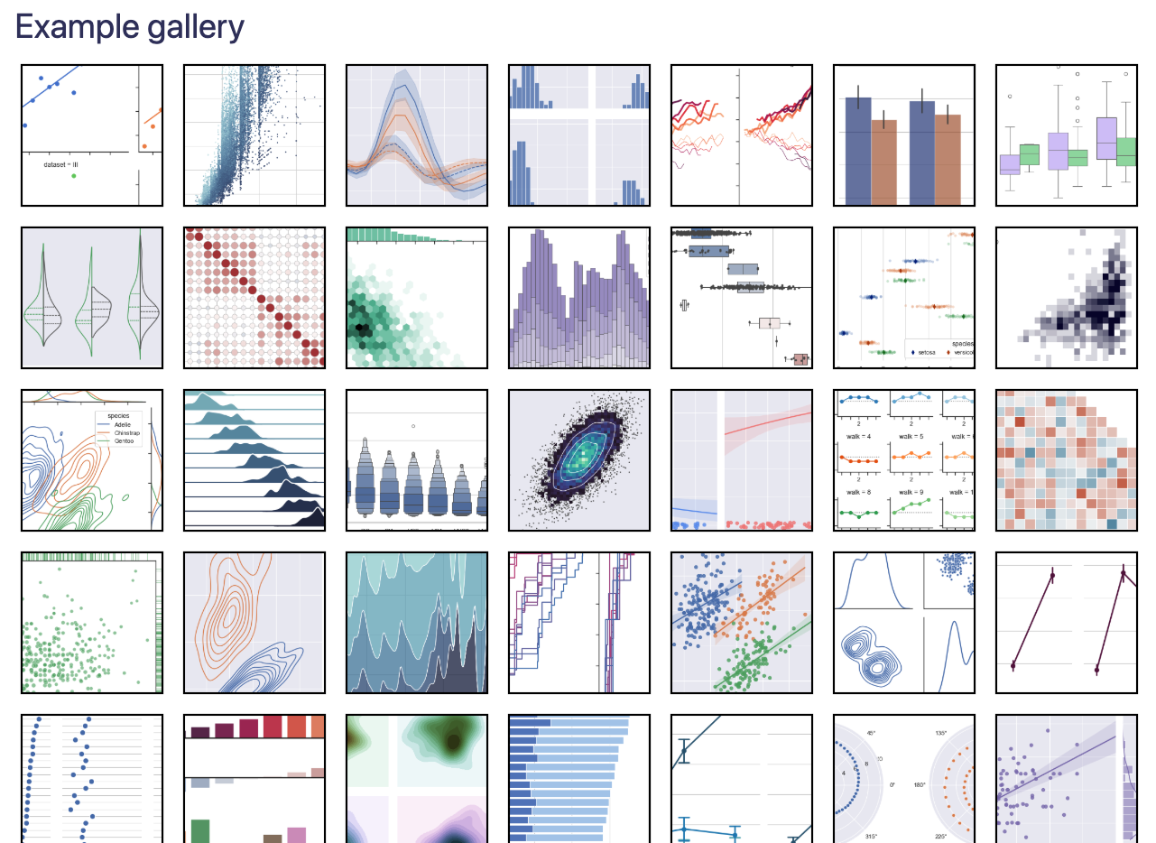
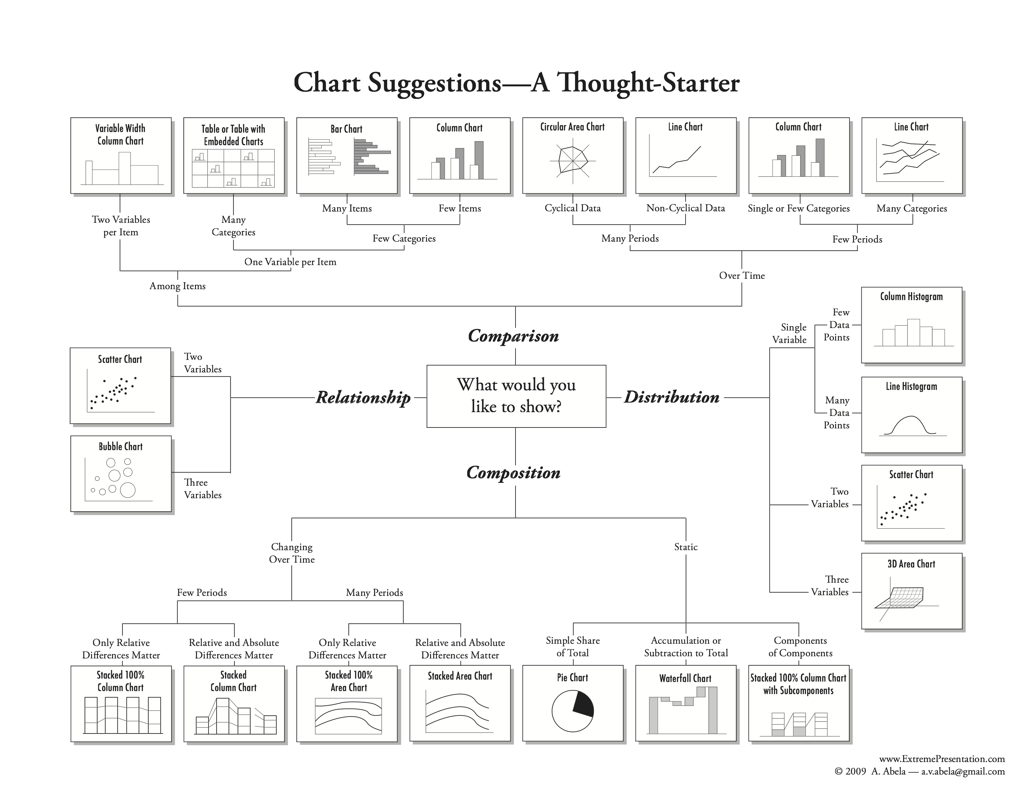
Chart type guide: relationship, comparison, distribution, composition

graphics don't always fall into neat taxonomies

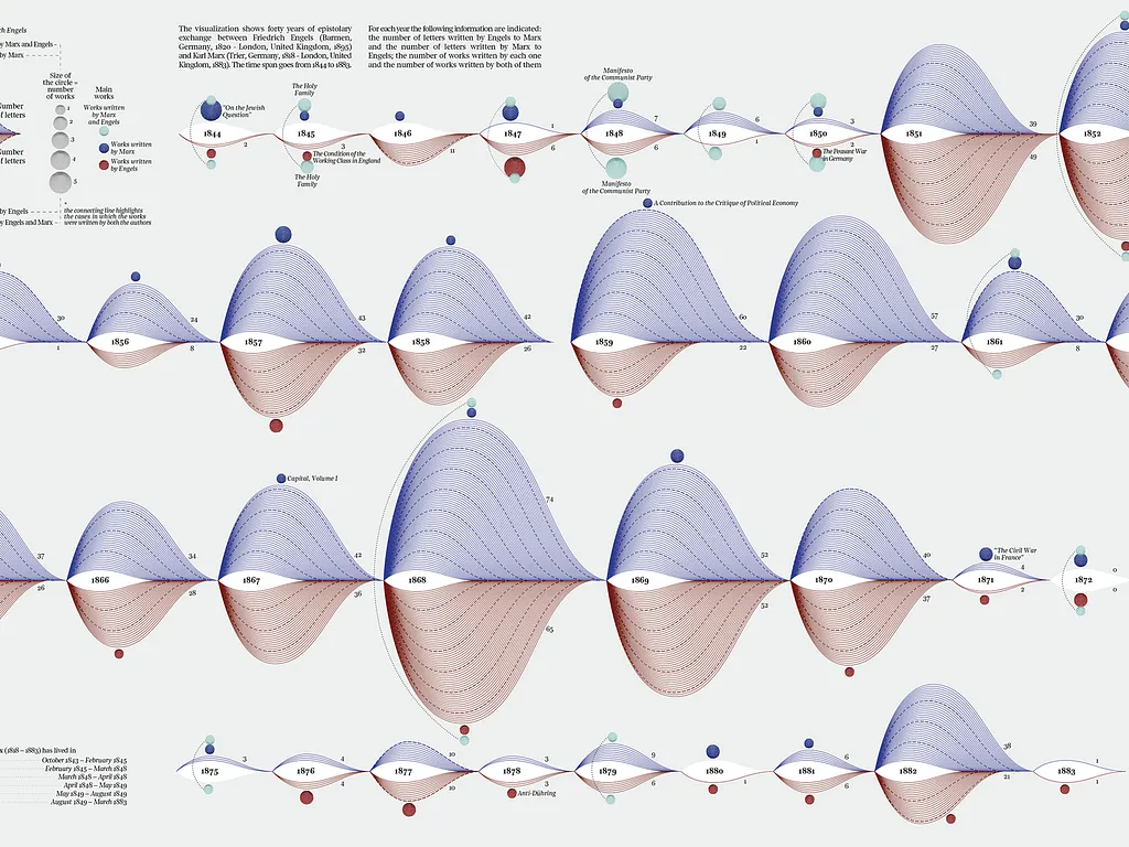
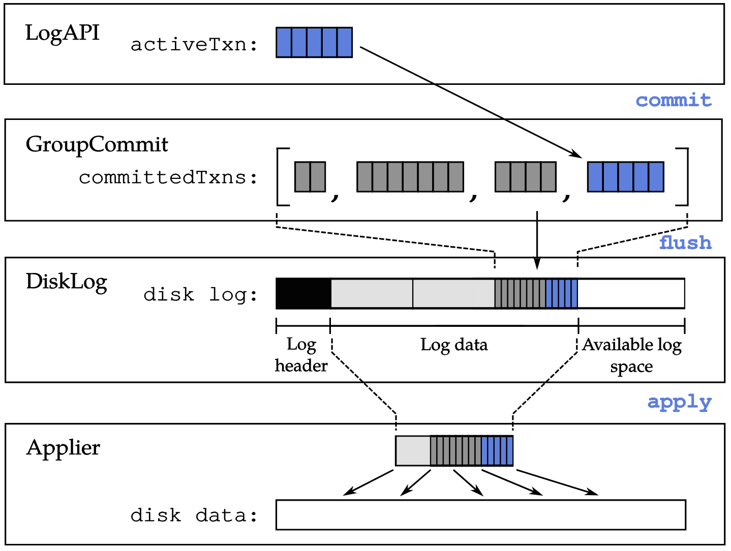
grouped bar charts aren't created equal

what trend do you see here?

what about now?

how about now?

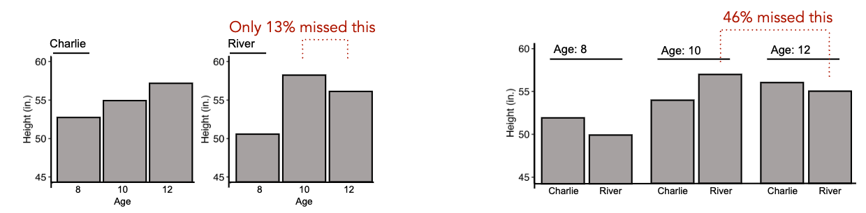
Boger and Franconeri study: separate bar charts vs grouped bars with participant miss rates

Boger & Franconeri 2024

these are all the same kind of chart — yet our takeaways differ

Key idea: when we design a graphic, we're doing more than picking a chart type. We're creating a visual structure for our readers to navigate.

data structure visual structure reader

The key idea of this talk is that when we're designing a graphic, we're doing a lot more than just picking a chart type — we're creating a visual structure for our readers to navigate. The way we arrange shapes and the colors we assign affect what our readers see first, what comparisons they make, and what story they take away.

In this talk you're going to see many examples of mapping data structures to visual structures to reader experiences. And through that process I'm gonna show you how thinking structurally frees you from this useful, but rigid lens of chart types and black-and-white design rules like banning pie charts, and helps you think more precisely and creatively about visualization.

To talk about visual structure precisely, we need a language.

GoFish
A compositional language for visual structure
open source (MIT-licensed), TypeScript with Python bindings (quickly catching up to TS)
See papers: UIST 2024, VIS 2025

GoFish is based on Gestalt grouping principles

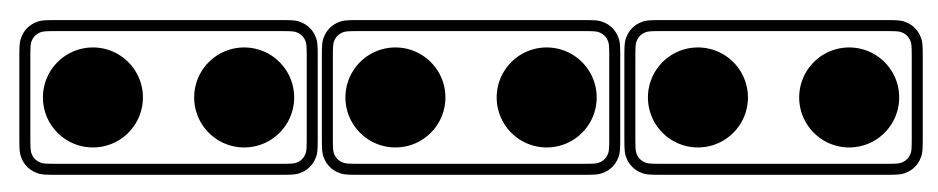
containment
connection
similar attribute
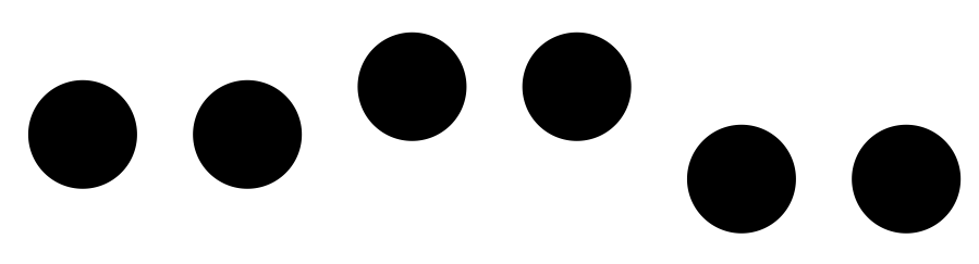
alignment
proximity / uniform density

containment
connection
similar attribute

alignment
proximity / uniform density

our first GoFish spec

chart(seafood)
    .flow(spread("lake", dir="x"))
    .mark(rect(h="count"))

chart(data) — attach your DataFrame

our first GoFish spec

chart(seafood)
    .flow(spread("lake", dir="x"))
    .mark(rect(h="count"))

.flow() — graphical operators arrange data into positions in space

our first GoFish spec

chart(seafood)
    .flow(spread("lake", dir="x"))
    .mark(rect(h="count"))

.mark() — what shape to draw at each position, and what channels to encode

Queries:

greatest / least total catch across lakes
pairwise comparison between any two lakes

part-to-whole relationships

→

`stack()`

chart(data).flow(
    spread("lake",    dir="x"),
).mark(
    rect(h="count")
)

chart(data).flow(
    spread("lake",    dir="x"),
    stack("species",  dir="y"),
).mark(
    rect(
        h="count",
        fill="species",
    )
)

chart(data).flow( # operators can be chained!
    spread("lake",    dir="x"),
    stack("species",  dir="y"),
).mark(
    rect(
        h="count",
        fill="species",
    )
)

Queries:

greatest/least lake total
pairwise lake comparisons
part-to-whole species comparisons (e.g., what % of Lake A is Bass?)
pairwise comparisons of the same species across lakes

lake → species (part to whole)

nesting order matters

                  lake → species
                  (part to whole)
                

chart(data).flow(
  spread("lake",    dir="x"),
  stack("species",  dir="y"),
).mark(rect(h="count", fill="species"))

                  lake → species
                

chart(data).flow(
  spread("lake",    dir="x"),
  spread("species", dir="x"),
).mark(rect(h="count", fill="species"))

                  species → lake
                

chart(data).flow(
  spread("species", dir="x"),
  spread("lake",    dir="x"),
).mark(rect(h="count", fill="species"))

flattening the hierarchy

                  lake → species
                  (part to whole)
                

chart(data).flow(
  spread("lake",    dir="x"),
  stack("species",  dir="y"),
).mark(rect(h="count", fill="species"))

                  lake × species
                

chart(data).flow(
  table("lake", "species"),
).mark(rect(fill="count"))

sorting keys

→

`derive()` to sort

chart(data).flow(
    spread("lake",   dir="x"),
    derive(lambda d: sorted(d, key="count")),
    stack("species", dir="y"),
).mark(
    rect(h="count", fill="species")
)

Queries:

greatest/least lake total
pairwise lake comparisons
greatest/least species total within lake
part-to-whole species comparisons (e.g., what % of Lake A is Bass?)
pairwise comparisons of the same species across lakes

connect across groups

→

connect the stacks into a continuous ribbon

chart(data).flow(
    spread("lake",   dir="x"),
    derive(lambda d: sorted(d, key="count")),
    stack("species", dir="y"),
).mark(
    rect(h="count", fill="species")
)

chart(data).flow(
    spread("lake", dir="x", spacing=64),
    derive(lambda d: sorted(d, key="count")),
    stack("species", dir="y"),
).mark(
    rect(h="count", fill="species")
)

Layer([
  chart(data).flow(
      spread("lake", dir="x", spacing=64),
      derive(lambda d: sorted(d, key="count")),
      stack("species", dir="y"),
  ).mark(
      rect(h="count", fill="species")
  ),
])

Layer([
  chart(data).flow(
      spread("lake", dir="x", spacing=64),
      derive(lambda d: sorted(d, key="count")),
      stack("species", dir="y"),
  ).mark(
      rect(h="count", fill="species").name("bars")
  ),
])

Layer([
  chart(data).flow(
      spread("lake", dir="x", spacing=64),
      derive(lambda d: sorted(d, key="count")),
      stack("species", dir="y"),
  ).mark(
      rect(h="count", fill="species").name("bars")
  ),
  chart(???).flow(???).mark(???),
])

Layer([
  chart(data).flow(
      spread("lake", dir="x", spacing=64),
      derive(lambda d: sorted(d, key="count")),
      stack("species", dir="y"),
  ).mark(
      rect(h="count", fill="species").name("bars")
  ),
  chart(select("bars")).flow(???).mark(???),
])

Layer([
  chart(data).flow(
      spread("lake", dir="x", spacing=64),
      derive(lambda d: sorted(d, key="count")),
      stack("species", dir="y"),
  ).mark(
      rect(h="count", fill="species").name("bars")
  ),
  chart(select("bars")).flow(group("species")).mark(???),
])

Layer([
  chart(data).flow(
      spread("lake", dir="x", spacing=64),
      derive(lambda d: sorted(d, key="count")),
      stack("species", dir="y"),
  ).mark(
      rect(h="count", fill="species").name("bars")
  ),
  chart(select("bars"))
    .flow(group("species"))
    .mark(area(opacity=0.8)),
])

Layer([
  chart(data).flow(
      spread("lake", dir="x", spacing=64),
      derive(lambda d: sorted(d, key="count")),
      stack("species", dir="y"),
  ).mark(
      rect(h="count", fill="species").name("bars")
  ),
  chart(select("bars"))
    .flow(group("species"))
    .mark(area(opacity=0.8)),
])

                  select("bars") =

                  [

                    { lake:
                  "Lake A", species:
                  "Trout", count:
                  31, __ref:
                  <GoFishMark> },

                    { lake:
                  "Lake A", species:
                  "Bass",  count:
                  23, __ref:
                  <GoFishMark> },

                    ...

                  ]
                

steering attention with color

→

`palette()` for discrete colors

Layer([
  Chart(data, color=palette({
      "Salmon": "#e15759",
      "Trout":  "#4e79a7",
  })).flow(
    spread("lake", dir="x", spacing=64),
    derive(lambda d: sorted(d, key="count")),
    stack("species", dir="y"),
  ).mark(
    rect(h="count", fill="species").name("bars")
  ),
  chart(select("bars"))
    .flow(group("species"))
    .mark(area(opacity=0.6)),
])

Color can promote and demote queries very precisely.

Salmon and Trout read as the main story across lakes. Queries about grayed-out species are de-emphasized. Some queries become impossible!

wrap into polar coordinates

Layer({"coord": clock()}, [   # ← one change
  Chart(data, color=palette({
      "Salmon": "#e15759",
      "Trout":  "#4e79a7",
  })).flow(
    spread("lake", dir="x",
           spacing=2π/6, mode="center"),
    derive(lambda d: sorted(d, key="count")),
    stack("species", dir="y"),
  ).mark(
    rect(w=0.1, h="count", fill="species").name("bars")
  ),
  chart(select("bars"))
    .flow(group("species"))
    .mark(area(opacity=0.6)),
])

This use of polar space makes many queries very hard. Only a few queries are afforded, like Trout starting high, crossing, Salmon, and ending low. Vice versa for Salmon.

mapping length to angle changes the afforded queries

pie

bar

Fine-grained comparison is MUCH harder

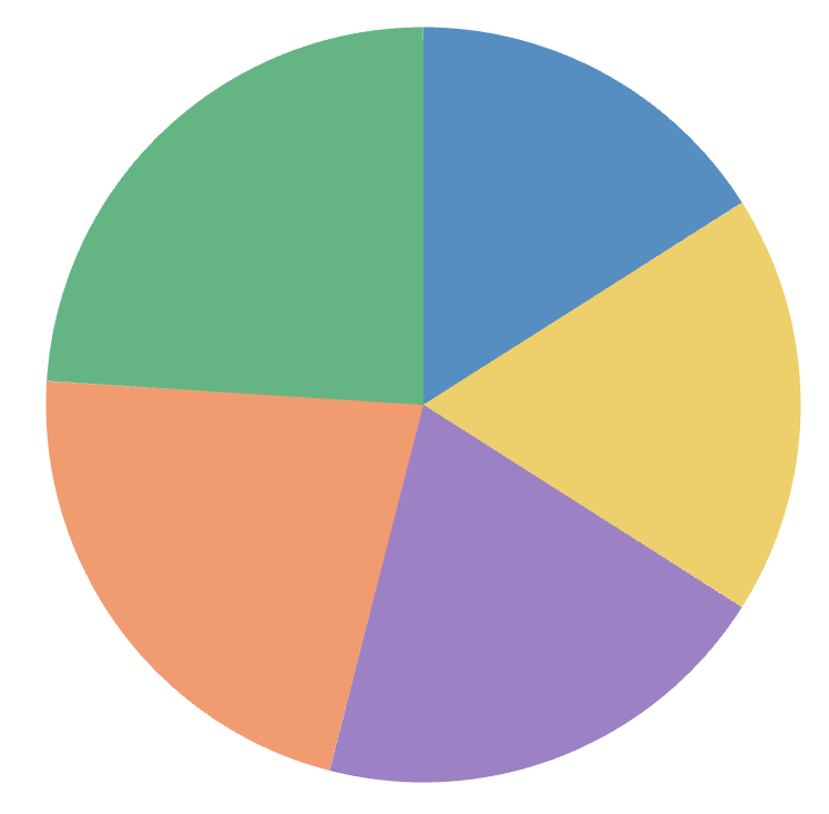
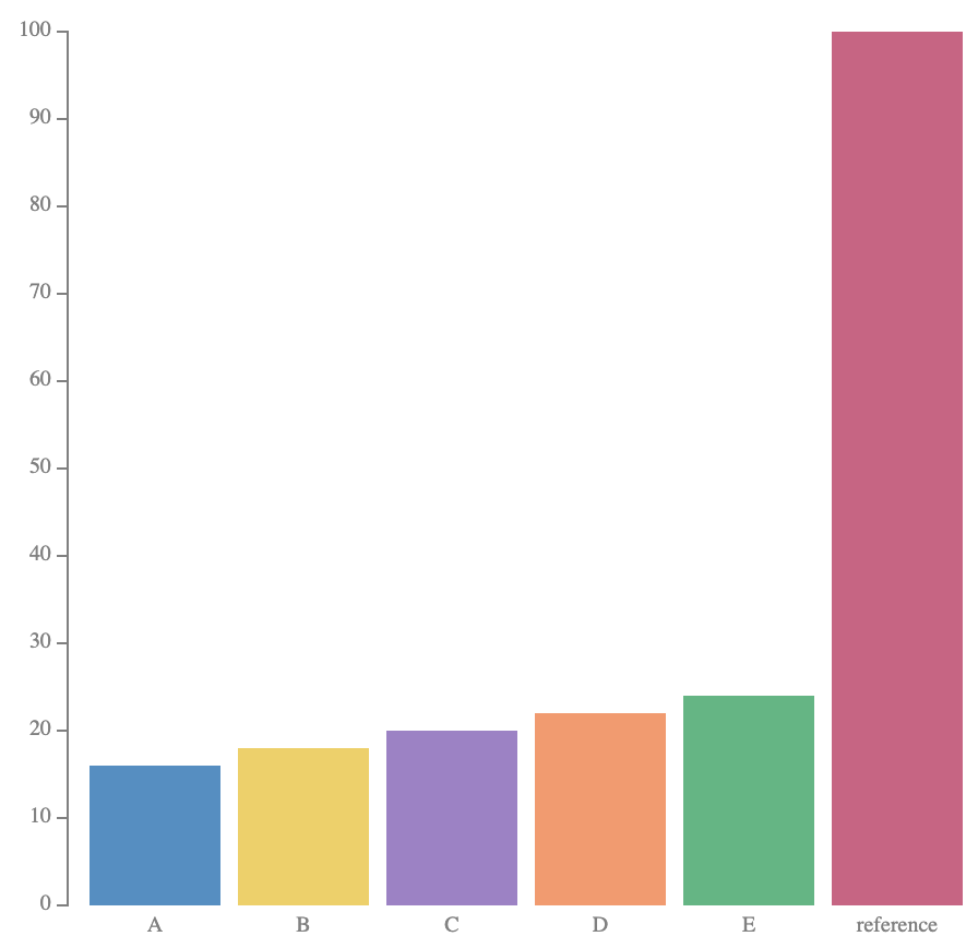
mapping length to angle changes the afforded queries

pie

bar

But coarse part-to-whole comparisons are much easier!

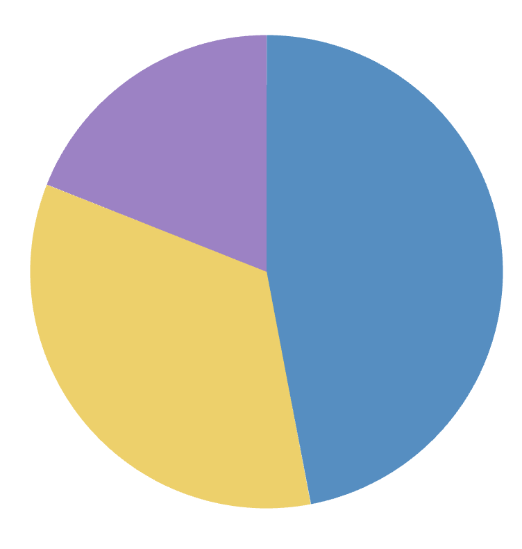
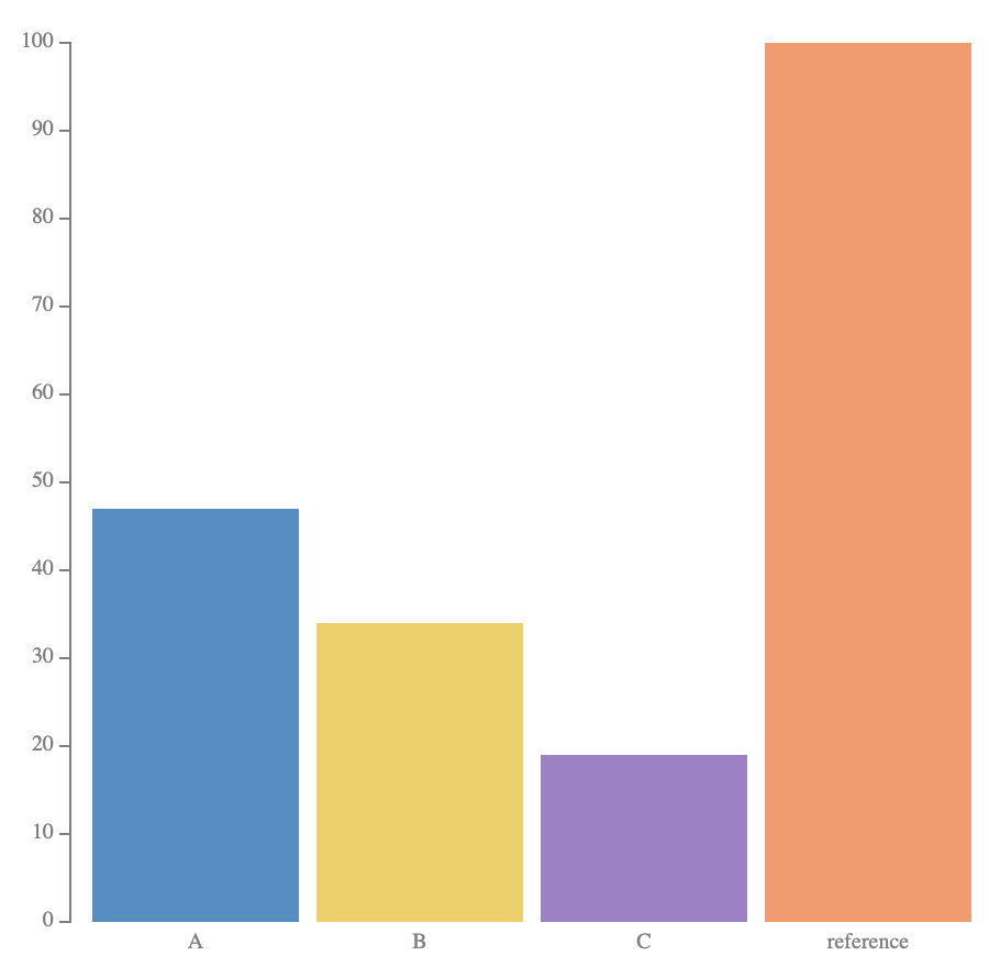
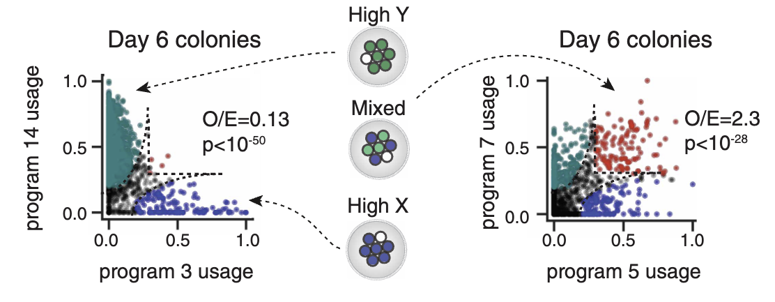
scatter -> pie = scatterpie

chart(scatter_data).flow(
    scatter("lake", x="x", y="y")
).mark(
    chart(coord=clock())
    .flow(stack("species", dir="x"))
    .mark(rect(w="count", fill="species"))
)

Outer structure: scatter() affords "where?" queries.

Inner structure: pie affords "what fraction?" queries.

Queries:

which species dominates each lake? (largest slice)
how does species composition vary across geography?
which lakes have similar mixes? (visual comparison)

Swap the inner chart for a different part-to-whole viz

chart(scatter_data).flow(
    scatter("lake", x="x", y="y")
).mark(
    Flower(...)
)

balloons???

chart(scatter_data).flow(
    scatter("lake", x="x", y="y")
).mark(
    Balloon(...)
)

When we think with structure instead of chart types, we can compose structures to come up with new designs while still reasoning precisely about what they communicate.

What just happened?

We took one dataset and made a series of deliberate structural moves.

Each move changed what was easy or hard to see.

We didn't have to pick from a menu of charts... though those are useful shorthands for common structures!

Instead, chart type labels like bar or pie were just structural motifs we encountered along the way.

operators map data types to Gestalt relations

Operator	Data type	Gestalt relation
`spread`	discrete	alignment & uniform density
`stack`	partitioned continuous	part-to-whole
`scatter`	continuous × continuous	none — no discrete grouping
`area / line / ribbon`	continuous or contiguous	connection
`table`	discrete × discrete	uniform density

takeaways

1. Chart types are great shortcuts, but graphics are really sophisticated visual structures.

2. Changing this structure changes what your reader can and can't see in (probably) predictable ways.

3. Thinking structurally helps us move beyond familiar charts and rigid rules to designs that might better fit our data or task.

Try it

$pip install gofish-graphics

Python alpha release coming soon!

🌐 Docs: gofish.graphics

🐙 GitHub: gofish-graphics/gofish-graphics

stay in the loop

buttondown.com/jopo

GoFish updates & new features
(~weekly)

Sneak peeks from the book on
designing better graphics
(longer cycles)

how do we decide what chart to use?

graphics don't always fall into neat taxonomies

grouped bar charts aren't created equal

what trend do you see here?

what about now?

how about now?

these are all the same kind of chart — yet our takeaways differ

GoFish is based on Gestalt grouping principles

our first GoFish spec

our first GoFish spec

our first GoFish spec

part-to-whole relationships

stack()

nesting order matters

flattening the hierarchy

sorting keys

derive() to sort

connect across groups

connect the stacks into a continuous ribbon

steering attention with color

palette() for discrete colors

wrap into polar coordinates

mapping length to angle changes the afforded queries

mapping length to angle changes the afforded queries

scatter -> pie = scatterpie

Swap the inner chart for a different part-to-whole viz

balloons???

What just happened?

operators map data types to Gestalt relations

takeaways

Try it

stay in the loop

`stack()`

`derive()` to sort

`palette()` for discrete colors