GoFish: Graphical Structure in Plain Sight

Josh Pollock with Arvind Satyanarayan

you can one-shot a dashboard now

*Sped up 2–4×; actual time ~2.5 min. Placeholder: Arvind's VizChitra demo, to re-record with a scientific dataset.

…or even a scrollytelling narrative

*Actual time ~15 min. Placeholder: Arvind's VizChitra demo.

The catch

ok, but is it actually good?

How do you know the figure shows what your reader needs? How do you know what you want in the first place?

For a scientific figure, "impressive" isn't the bar. The bar is: does it support the comparisons your argument depends on?

The way out

we need to see structure, not chart types

To judge a figure, yours or the AI's, you need a way to see what it's doing.

Not "which chart type is this?" but "what does this arrangement let my reader see?"

start with the lakes

The examples use fishery data: lakes, species, catch amounts, and locations.

That matters because the data are naturally relational. We care about parts and wholes, where things happened, and how the same species moves through several views.

how do we decide what chart to use?

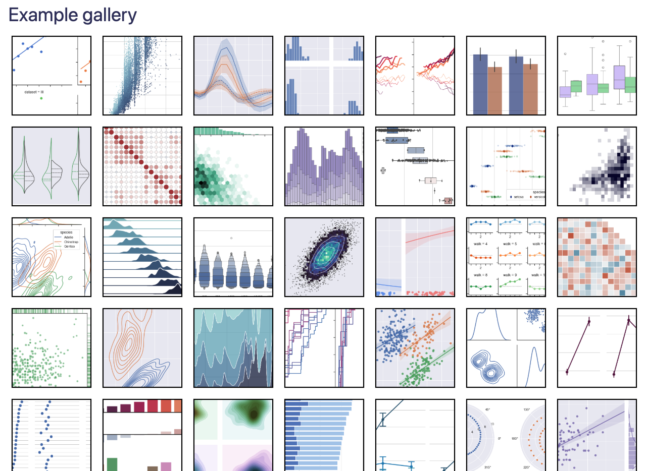
chart types lack underlying structure

how do we decide what chart to use?

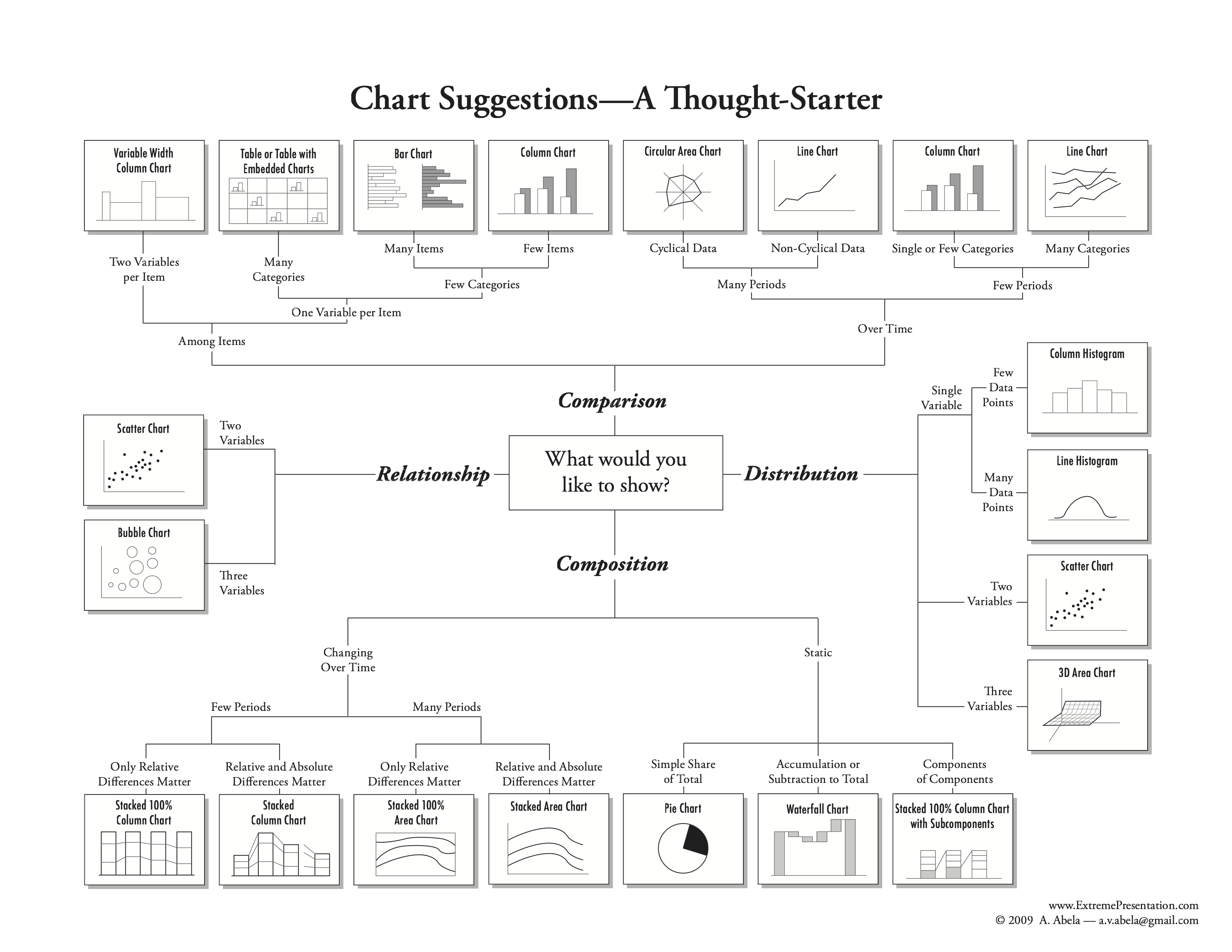
Chart type guide: relationship, comparison, distribution, composition

task taxonomies are vague

how do we decide what chart to use?

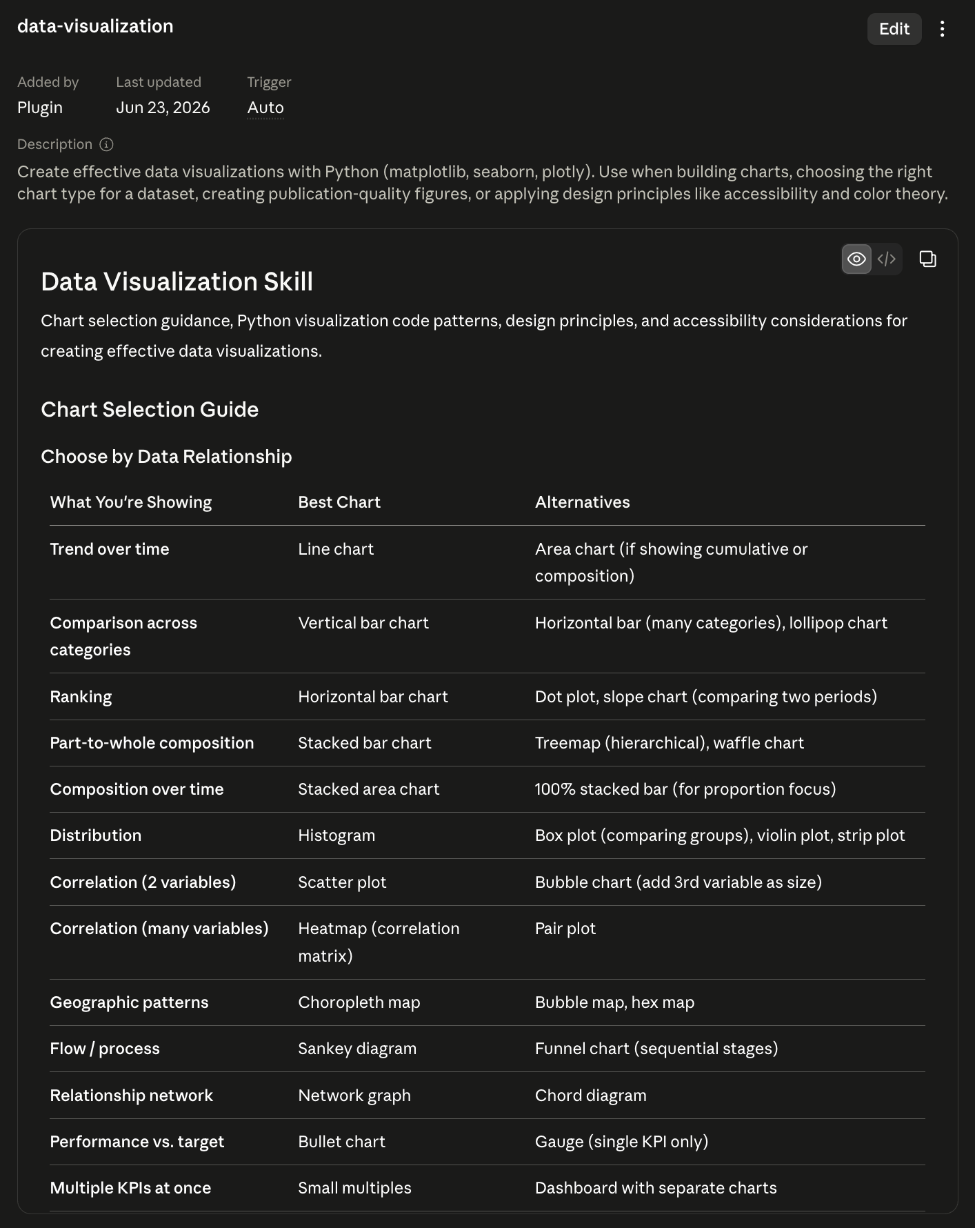
Screenshot of Claude's data-visualization skill file, a task-to-chart-type lookup table

ossified into AI skills

And the third answer: most of you are already using AI agents to make your figures, and they're genuinely good at the implementation, writing the code was never going to stay the bottleneck. The problem that remains is picking the graphic you want, judging whether it's good, and steering the design. And here's the catch: this is the actual skill file Claude uses for visualization, a table mapping coarse task descriptions to chart types. The chart picker didn't go away, the chart types and the task taxonomies are getting ossified into AI skills, not improved. And because the conventional chart types are where the training data is, the agent quietly pulls every figure toward the mean. Judging the output, and knowing what to ask for, is now the whole game.

The problem

menus become rules

This chart is good. This chart is bad. Use this color scheme, not that one.

Rules are useful, but brittle. They tend to be all-or-nothing just when scientific graphics need judgment.

and often that's fine

but what about the long tail

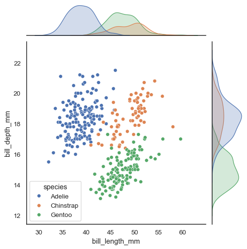
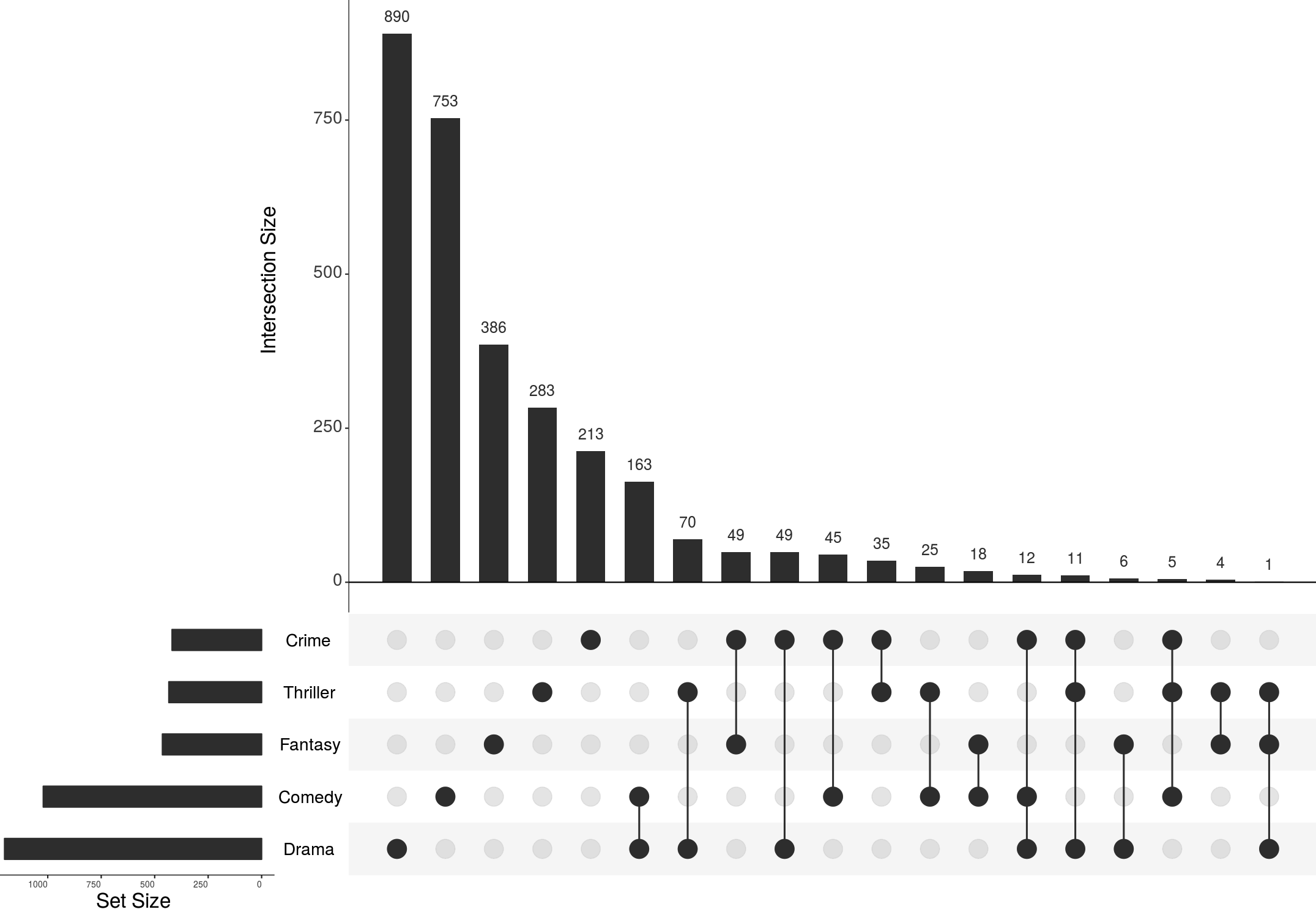
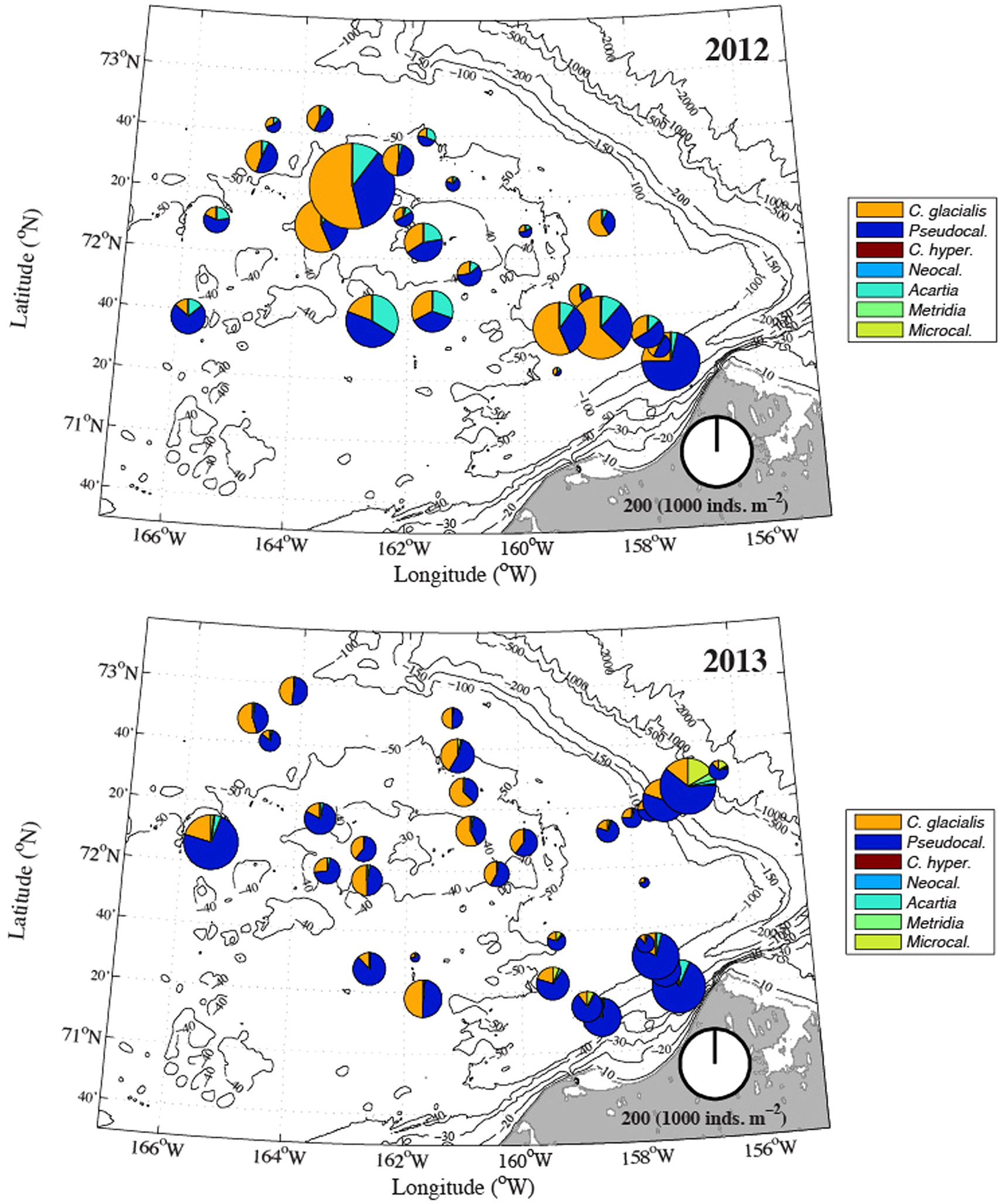
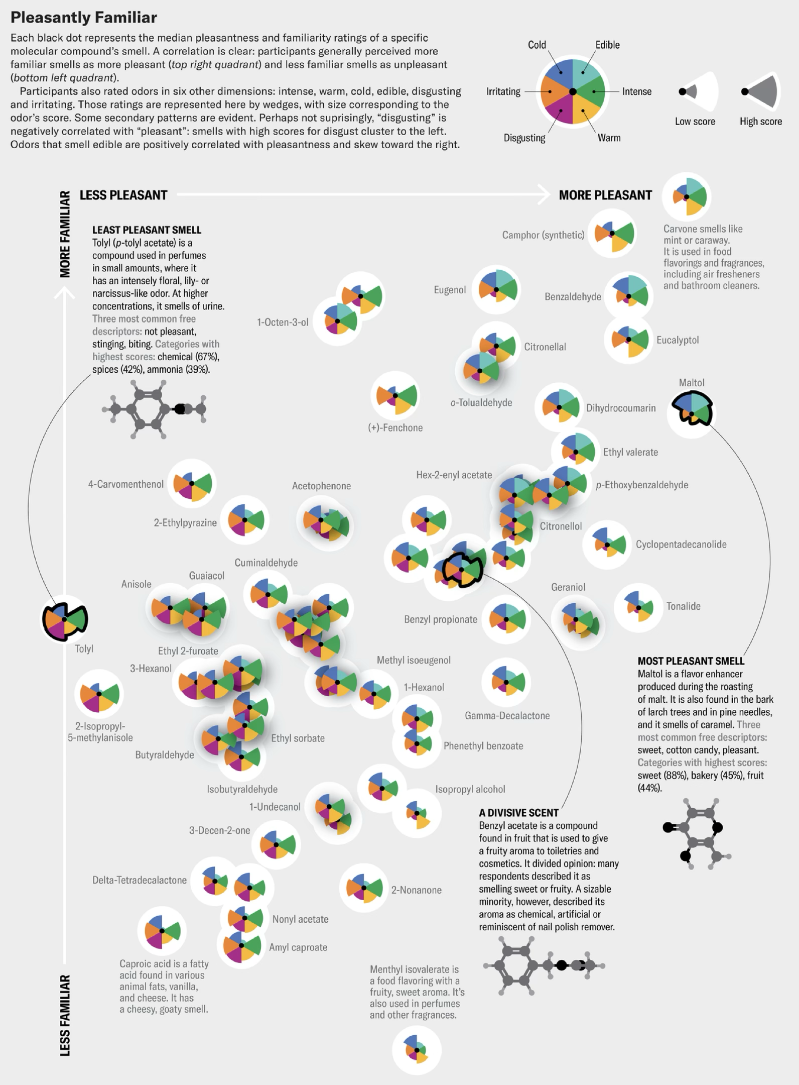
Jen Christiansen's scatterplot of coxcomb glyphs, Scientific American

how do we figure out what to make?

how do we make it?

Look at the graphics scientists actually use and publish. A Seaborn jointplot; an UpSet plot; oceanographers plotting scatterplots of pie charts; Jen Christiansen in Scientific American with a scatterplot of coxcombs. These are bespoke, composite, long-tail graphics. What makes them work is how their pieces are arranged, the alignment between the marginals and the scatter, the positioning of glyphs in a shared space. None of that is on a picker menu, and "jointplot" won't be the name of the thing your paper needs next. And these graphics raise two questions. First: how do we even figure out what graphic to make in the first place? And second: once we know what we want, how do we actually make it?

The stance

I'm a stylistic anarchist

Not anti-style. Anti brittle rules.

A prerequisite to designing good graphics is seeing what they are doing as clearly as possible, before ranking them by type.

grammar vs elements of style

A better lens

Grammar names the relationships. Style controls the voice.

Grammar

containment, alignment, connection, order, scale, emphasis

Style

palette, texture, typography, density, ornament, tone

graphics don't always fall into neat taxonomies

here's a grouped bar chart

what did you notice about the data?

here's another one

what did you notice now?

what about now?

how about now?

chart(heights)
  .flow(
    spread(by="age", dir="x"),
    spread(by="person", dir="x")
  )
  .mark(rect(h="height", fill="person"))

Boger and Franconeri study: separate bar charts vs grouped bars with participant miss rates

Boger & Franconeri 2024

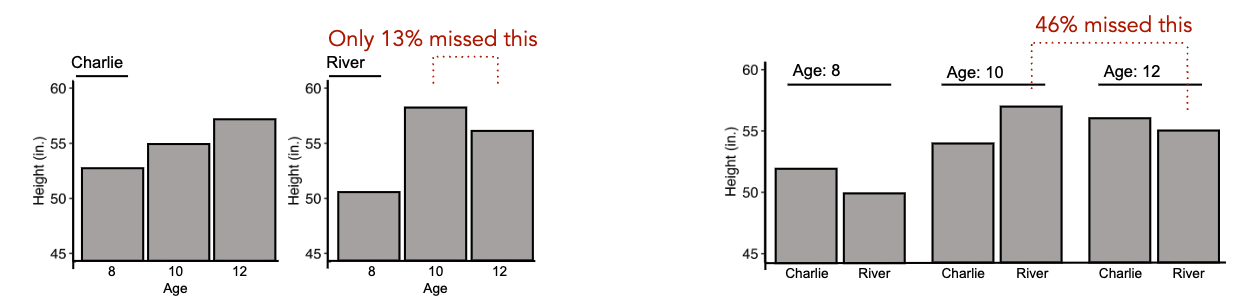
these are all grouped bar charts, but we read them differently!

by the way: this is real data

the grammar of graphics: marks, channels, and coordinates

marks (shapes)

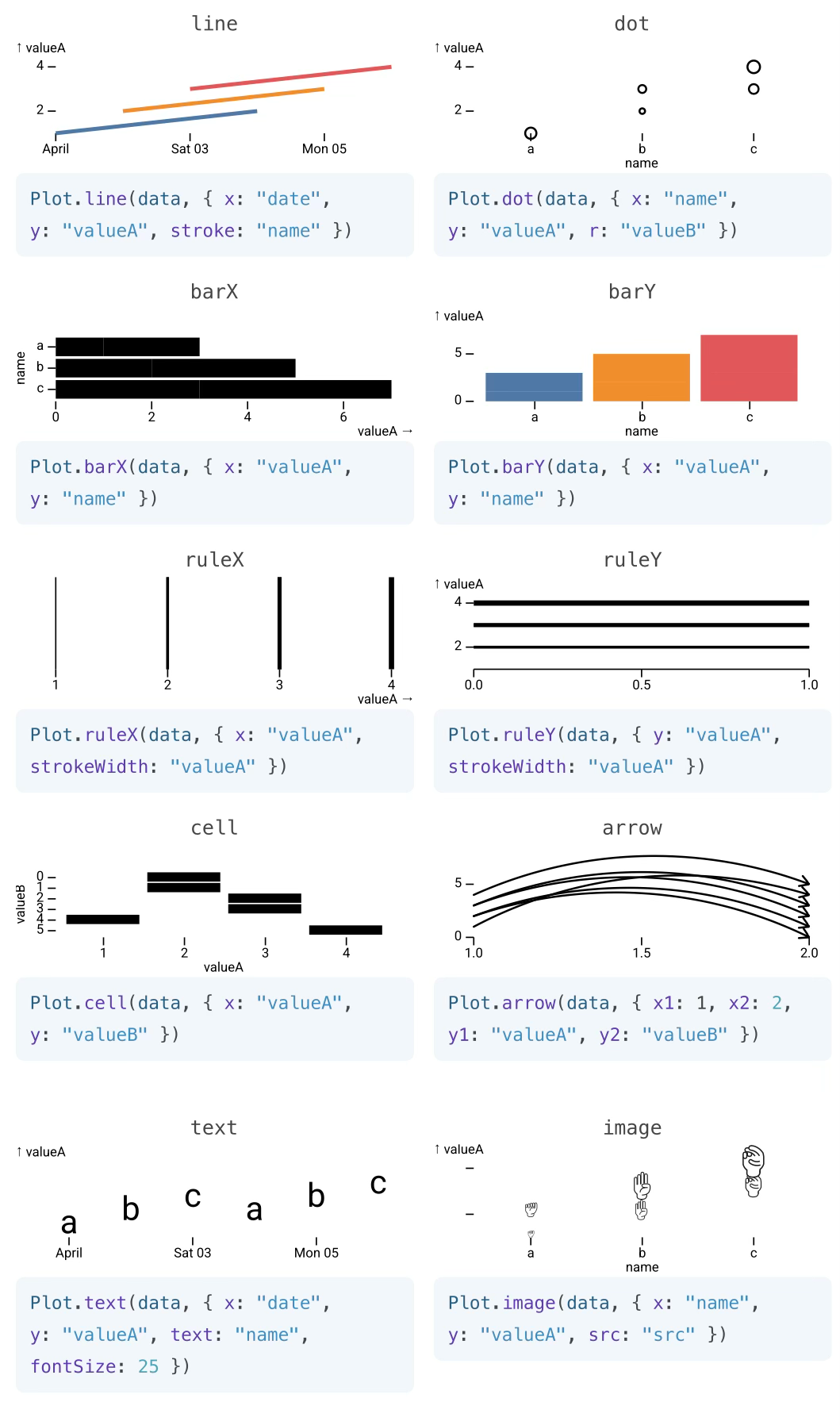
Observable Plot

channels (shape attributes)

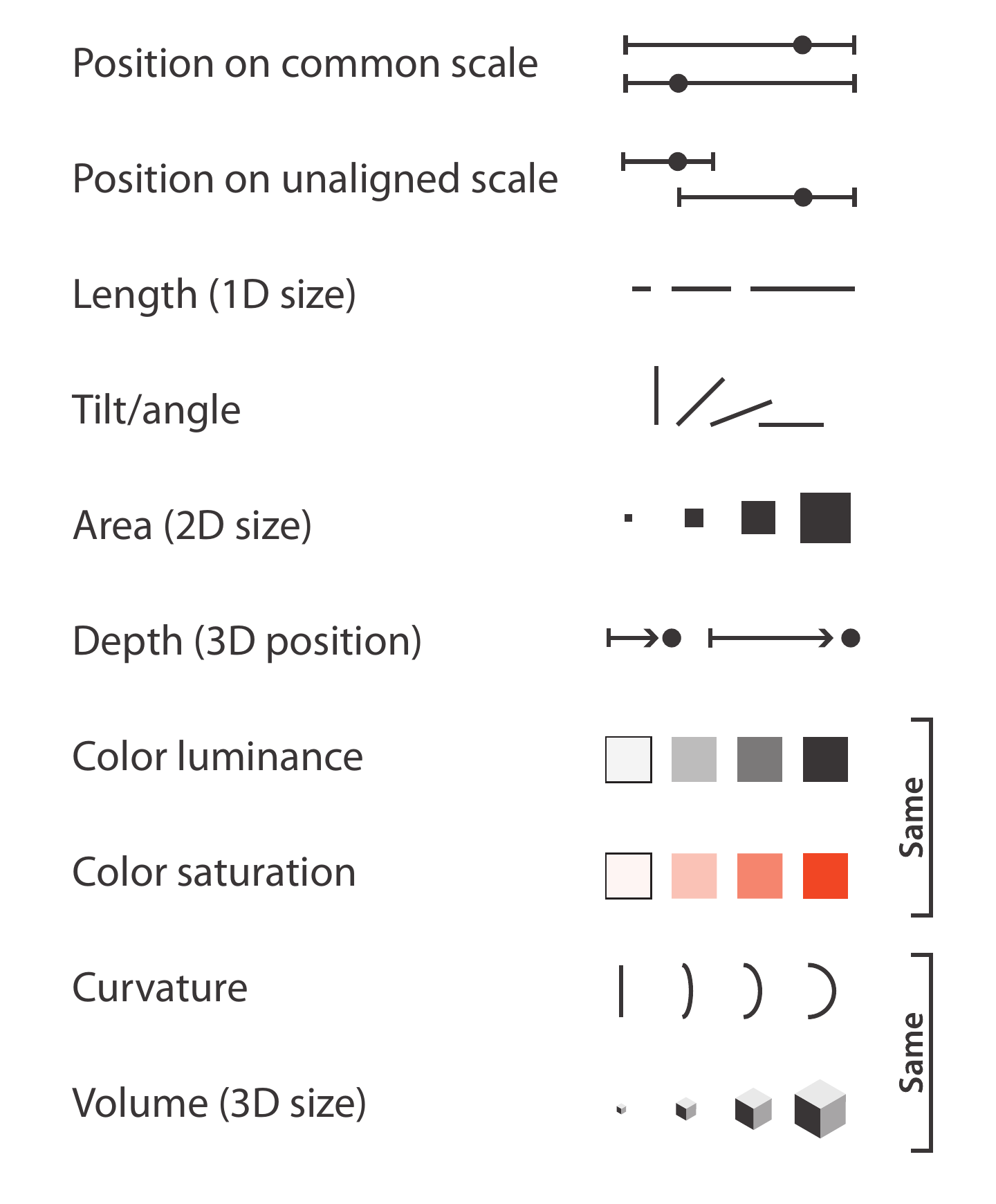
Munzner's ranking of visual channels by accuracy

Munzner, Visualization Analysis and Design (2014)

coordinates (space transformations)

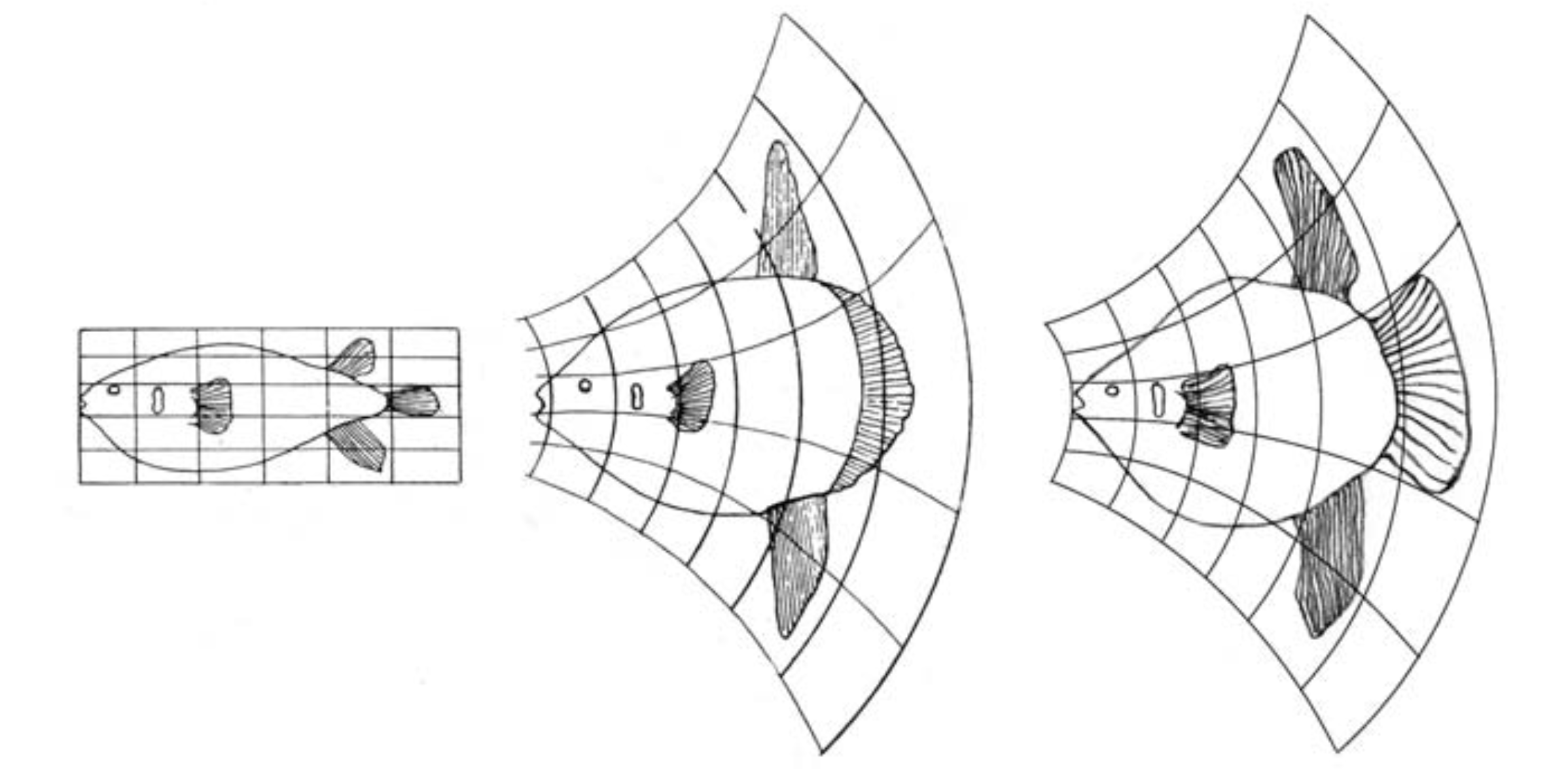
Thompson’s growth transformation: a fish and its coordinate grid progressively warped into two curved forms

Thompson’s growth transformation · via Wilkinson, The Grammar of Graphics

but we need a notion of visual structure to explain what we just saw

This is the strongest answer yet. You might object that the grammar of graphics already gives us first principles: marks and channels. Marks are the shapes; channels are how data maps onto them, and there's a famous accuracy ranking: position and length beat angle, area, and color. That tells us how precisely one value can be read. Coordinate systems can also transform the space in which those marks are drawn. But you just saw the counterexample: same marks, same channels, same rankings, and you read the three charts differently. Marks and channels are blind to arrangement and how things are grouped and laid out. So we need a way of talking about arrangement.

Marks and channels tell us how precisely to read a value. They don't tell us which questions a chart makes easy.

Key idea: when we design a graphic, we're doing more than picking a chart type. We're creating a visual structure for our readers to navigate.

data structure visual structure reader

The key idea of this talk is that when we're designing a graphic, we're doing a lot more than just picking a chart type, we're creating a visual structure for our readers to navigate. The way we arrange shapes and the colors we assign affect what our readers see first, what comparisons they make, and what story they take away.

In this talk you're going to see many examples of mapping data structures to visual structures to reader experiences. And through that process I'm gonna show you how thinking structurally frees you from this useful, but rigid lens of chart types and black-and-white design rules like banning pie charts, and helps you think more precisely and creatively about visualization.

graphics are visual data structures 🪾

GoFish
A compositional language for visual structure
open source (MIT-licensed), TypeScript with Python bindings (quickly catching up to TS)
See papers: UIST 2024, VIS 2025

that we query with our eyes 👀

structure changes what becomes easy to see

The whole talk in one sentence. A chart is not a picture of numbers, it is a data structure laid out in space, and reading it is running queries against that structure with your visual system. Structure is the first half. [advance] The structure language exists: GoFish, open source, alpha, you can install it today. It's the culmination of a PhD spent studying how visual structure conveys meaning and building better libraries to take advantage of it. The second half is what the structure lets your eyes do. You just experienced this: changing the grouping changed which comparison was immediate. Hold onto that practical idea. We do not need a formal query language to use it throughout the talk.

so we need two languages

1 · a language of graphical structure

GoFish
A compositional language for visual structure
open source (MIT-licensed), TypeScript with Python bindings (quickly catching up to TS)
See papers: UIST 2024, VIS 2025

2 · a language of perceptual queries

speculative, cutting-edge research. please push back!

GoFish

visual structure can help us describe both simple charts and very complex ones

familiar chart space

bar chart

slope chart

delta bars

the long tail

waffle

mosaic

ribbon

bottle chart

beyond chart space

sankey tree

Pulley diagram rendered with GoFish — pulley diagram

sunburst

Orthogonal node-link tree rendered with GoTree and GoFish — orthogonal tree

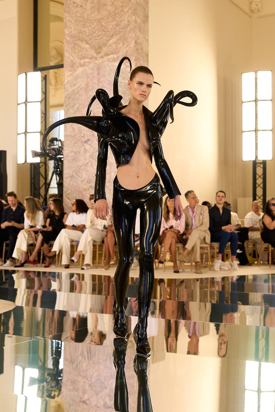
high fashion for graphics tools

Runway PL

Jean Yang asks what happens when programming-language ideas get the same public design culture that fashion has.

I want that for scientific figures: couture-level structure, made available for everyday chart decisions.

Jean Yang, “Runway PL” and Fast Fashion · Schiaparelli FW 2026-27

Schiaparelli Fall/Winter 2026-27 runway look with kinetic tentacle-like shoulders — Schiaparelli FW 2026-27

This opening is borrowing Jean Yang's runway PL framing: make the ideas behind programming languages feel like a design culture more people can enter. I looked for a fish-fashion reference and the strongest one is Schiaparelli Fall/Winter 2026-27, whose official collection notes describe a look encrusted with real fish scales and a palette drawn from sea fauna. The recent Louis Vuitton Spring/Summer 2027 menswear show also had the giant artificial wave set, but Schiaparelli gives us the tighter bridge: fish, couture, structure, and technique. Source links: https://jeanstack.substack.com/p/runway-pl-and-fast-fashion and https://schiaparelli.com/en/pages/haute-couture-automne-hiver-2026-27

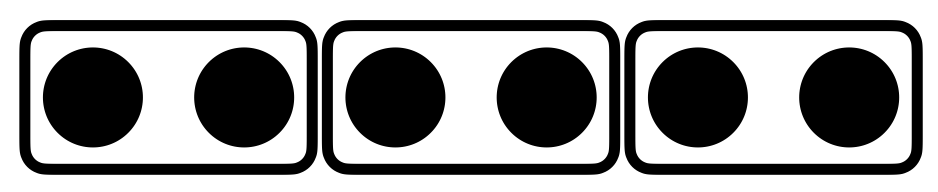
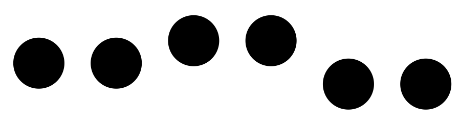
GoFish is based on Gestalt grouping principles

containment
connection
similar attribute
alignment
proximity / uniform density

containment
connection
similar attribute

alignment
proximity / uniform density

GoFish has three four API tiers

chart templates proposed

bar_chart(data, x="category", y="value")

popular chart types

pipelines

chart(data)
  .flow(spread(by="category", dir="x"))
  .mark(rect(h="value"))

common and uncommon statistical graphics

components

groups = (
  data.group_by("category")
      .agg(pl.col("value").sum())
)

rects = [
  rect(key=d["category"], h=datum(d["value"]))
  for d in groups.iter_rows(named=True)
]

spread(rects, dir="x", alignment="baseline")

one-off annotations, non-tabular data (e.g., trees)

constraints

groups = ...

rects = ...

layer(rects).constrain(lambda a, b, c: [
  Constraint.align([a, b, c], y="baseline"),
  Constraint.distribute([a, b, c], dir="x")
])

diagrams and other bespoke graphics

GoFish currently gives us three ways to describe the same structure. Pipelines are the everyday chart-building API. Components expose the visual tree directly. Constraints expose the relations that operators compile down to: align the bars at a common baseline, then distribute them along x.

These are not separate systems, and you do not have to choose one tier for an entire graphic. The tiers interoperate. A pipeline constructs components and elaborates into constraints; you can start at a high level, then drop down locally for one annotation, one non-tabular subtree, or one bespoke relation. The arrows are meant literally: each level expands into the level beneath it.

There is a proposed fourth tier above pipelines: chart templates. The design notes call these named expansions, not new primitives. So bar_chart is just a concise name for the pipeline immediately below it, and it remains possible to elaborate or customize the result at a lower tier. The dashed boundary marks this tier as a proposal rather than the stable API used in the rest of the talk. [advance] For the rest of this talk, we're going to work primarily at the pipeline tier.

back to those bar charts

                  spread by year, then by city
                

                  spread by city, then by year
                

start with the data shape

GoFish walkthrough

chart(barley)
  .flow(
  )
  .mark(
  )

operators marks data transforms

start with the data

chart(barley)

variety	site	year	yield
Manchuria	University Farm	1931	27.00
Manchuria	Waseca	1931	48.87
Manchuria	Morris	1931	27.43
…	…	…	…

place one slot per site

chart(barley)
  .flow(
    spread(by="site", dir="x")
  )

make yield visible

chart(barley)
  .flow(
    spread(by="site", dir="x")
  )
  .mark(
    rect(h="yield")
  )

some transforms are implied

chart(barley)
  .flow(
    spread(by="site", dir="x")
  )
  .mark(
    rect(h="yield")
  )

aggregate yield by site

add a second grouping

chart(barley)
  .flow(
    spread(by="site", dir="x"),
    spread(by="year", dir="x")
  )
  .mark(
    rect(h="yield", fill="site")
  )

data transformation pipeline

barley 120 rows variety · site · year · yield

↓ group_by("site")

University Farm20 rows

Waseca20 rows

…

Morris20 rows

↓ group_by("year")

19311932

…

19311932

↓

rect rect

…

rect rect

each rect h = sum(yield) fill = first(site)

each line of the spec is a cut

chart(barley).flow(
  spread(by="site", dir="x"),
  spread(by="year", dir="x"),
).mark(rect(h="yield", fill="site"))

compare ⟨each site's year pattern⟩ across sites

site = Morris compare ⟨yield heights⟩ across years

site = Morris · year = 1932 yield → height · site → color

Highlighting a line of the spec picks a CUT through the operator tree, Elmqvist-style hierarchical aggregation, but the cut is wherever your eye lands in the code, not a fixed level someone baked into the chart. We start at the very bottom of the spec, the mark line, so the cut sits as low as it can go: the boundary is a single bar, and there is nothing below the cut left to collapse into a summary glyph, because the mark is the leaf, this first step is the one place in the whole sequence where nothing is hidden. The focused region is marked by a drawn dashed boundary around the bar in play rather than by graying out the rest, this slide has earned the right to use its own machinery: common region is the strong Gestalt cue (the whole reason grouping/adjacency reads as comparison at all), where dimming was only ever a salience nudge borrowed for the earlier Boulder slide back in the opening. Watch the boundary as the steps advance: right now it hugs a single bar, as small as it can get, and it will grow one enclosure at a time as the cut moves up the spec, first to Morris's pair of bars, then to the entire plot. The chip states that same story directly: the header is a full set of concrete field = value bindings (site = Morris, year = 1932), every coordinate is pinned down, so there's no hole in the query body, just a direct channel mapping, yield → height, site → color. With nothing left to search for and nothing to aggregate, the query degrades to the cheapest thing on the menu: a lookup. As the cut moves up from here, a binding will leave the header, a hole will open where it used to be, and that hole is what the next slide's notation is for. The chip that just landed isn't alone on the slide by accident: it's the bottom of a column, and that column will grow upward one chip at a time as the cut climbs the spec, so that by the top step every line of code has its chip sitting beside it at once.

each line of the spec is a cut

chart(barley).flow(
  spread(by="site", dir="x"),
  spread(by="year", dir="x"),
).mark(rect(h="yield", fill="site"))

compare ⟨each site's year pattern⟩ across sites

site = Morris compare ⟨yield heights⟩ across years

site = Morris · year = 1932 yield → height · site → color

One line up: the cut moves off the mark and onto the inner spread(by="year"), and the mark line itself drops below the cut for the first time. Below the cut, the tree collapses into a summary glyph: this is just the inner substitution GoFish already does whenever a grouping level is left out of a spec, the same auto-summing behind "back to those bar charts." Concretely, on this step it happens site by site: every site other than Morris has its whole spread over years flattened down to one neutral gray bar of its total, while Morris, the one site the header pins down, stays exploded into its own bar per year, because that's what's inside the boundary now. So the visualization of the idea (fade what's below the cut into a summary) is itself an instance of the idea (a lower level of the spec, collapsed). The boundary grows to match: from a single bar up to Morris's whole pair of bars, one enclosure bigger than the mark step. The header shrinks the same amount it grew: year = 1932 is gone, discharged into the query body as "across years," and only site = Morris is left pinned down, boundary and header are the same widening cut, drawn vs. written. This is also where the perceptual-query notation is introduced properly for the first time: the hole in the chip, ⟨yield heights⟩, is a placeholder for the reader's own attention, marking what the boundary is now cheap enough to compare but hasn't been read out yet. The chip states the query; what it costs to actually run it is worth saying out loud rather than printing, here, bars sit adjacent, so the estimate is cheap: one glance, not a verdict on whether the chart is good, just what this arrangement charges for the comparison. A second chip has now landed above the first, and it's not floating free, it sits directly beside the spread(by="year") line, the way the mark chip below it sits beside the mark line, so the column is starting to read like a legend for the spec itself. Worth noticing in passing: the header just got shorter than the mark chip's, one binding lighter, because year = 1932 dropped out of the address and reappeared as "across years" in the body, that's the same shrink the boundary talk above is describing, just visible in the chip stack now too.

each line of the spec is a cut

chart(barley).flow(
  spread(by="site", dir="x"),
  spread(by="year", dir="x"),
).mark(rect(h="yield", fill="site"))

compare ⟨each site's year pattern⟩ across sites

site = Morris compare ⟨yield heights⟩ across years

site = Morris · year = 1932 yield → height · site → color

search, where is it? look up find follow look up: you were handed the address. find: you weren't, the chart has to make the answer visible. follow: trace a link. query, what about it? read compare collect read: decode one value or event. compare: relate two or more located things. collect: summarize all of them.

One more line up, and we're at the top of the spec: the cut moves onto the outer spread(by="site"), and now the year line collapses too, along with the mark line beneath it, both fall below the cut, both fold into summary glyphs wherever the layout doesn't need them expanded. The boundary takes its last, biggest step: from Morris's pair of bars out to the entire plot, every site now participating, nothing held back as a special case anymore. The header shrinks to match, and this time it empties out completely, there's no field = value binding left to write, because we're no longer looking at one example region, we're looking at all of them at once. That's exactly what the query body says without any header at all: ⟨each site's year pattern⟩, compared across sites. All three chips are up now, and the column next to the spec is the whole claim of this slide's title made literal: read down the column and you're reading down the spec, one chip per line, in the same order. Read it top to bottom and two things move in opposite directions, the headers thin out as you go up, a full site = Morris · year = 1932 address at the bottom, down to site = Morris with year gone, down to no header at all at the top, while the holes do the opposite, growing from nothing, to a hole, to a whole shape. And the cost tracks both: a lookup at the bottom, a glance in the middle, a scan at the top. Three chips, three prices, one spec. The hole is bigger than either of the last two steps' holes, it's not one number, it's a whole shape, repeated once per site, and it's worth pricing that out loud: groups sitting apart is a real perceptual act, but reading ten of them side by side is a scan, the most expensive query in this three-step arc. Lookup, then one glance, then a scan, the query gets more expensive exactly as the boundary gets bigger and the header gets emptier; three prices for the same widening cut. The key underneath the chip spells out the six verbs the chips use, and they aren't arbitrary, they split into two tiers. Look up, find, and follow are all "where is it" questions: look up means someone handed you the address (a key, a coordinate) and the index just retrieves it; find means there is no address, you're hunting, and the chart has to make the answer visible; follow means tracing a link, like a line or a ribbon. Read, compare, and collect are all "what about it" questions once you're already looking at the right place: read decodes one value, compare relates two or more things you've found, collect summarizes the whole crowd at once. Worth saying out loud later, when the delta-bars slides come up: that whole four-step arc is the story of turning a find into something close to a look up. Early on, "which way did yield move at this site" is a real hunt, you have to read a line's slope, one of ten per panel, and there's no shortcut. By the time the bars are diverging from a zero baseline, the sign has an address: which side of the baseline the bar falls on. The audience isn't searching anymore, they're just looking. Same query the whole way through, priced cheaper and cheaper.

group by site, then year

chart(barley).flow(
  spread(by="site", dir="x"),
  spread(by="year", dir="x"),
).mark(rect(h="yield", fill="site"))

compare ⟨each site's year pattern⟩ across sites

site = Morris compare ⟨yield heights⟩ across years

site = Morris · year = 1932 yield → height · site → color

site → year: each site's two years sit together, so the change per site is easy to read. Now that the chips are all up at once, here's what that adjacency buys: the top chip's hole is ⟨each site's year pattern⟩, compared across sites, and it's nesting by site first that puts each site's two years right next to each other, which is the only reason "each site's year pattern" is a single readable shape instead of two bars you'd have to go find on opposite sides of the plot. The middle chip zooms into one site and prices the within-site comparison as a glance, Morris's two years, side by side. The bottom chip is the same lookup it always was: one rect, one color. Same three prices as the cut slides, but now all three are visible together, because there's no single cut being made here, the whole point of this slide is that all three queries are live at once, for this particular nesting order.

or group by year, then site

chart(barley).flow(
  spread(by="year", dir="x"),
  spread(by="site", dir="x"),
).mark(rect(h="yield", fill="site"))

compare ⟨each year's site pattern⟩ across years

year = 1932 compare ⟨yield heights⟩ across sites

year = 1932 · site = Morris yield → height · site → color

year → site: sites sit together within each year, so the per-site change is scattered across the two blocks. Same three chips as the last slide, same data, same operators, only the nesting order has flipped, and you can read that flip straight off the two chip columns if you compare them across this slide advance: same shape, top to bottom, but every site and year token has traded places. The hole at the top is now ⟨each year's site pattern⟩, compared across years, a scan, same as before, but the thing being scanned has changed from "one site's two years" to "one year's six sites." The middle chip zooms into a single year and prices the within-year comparison across sites as a glance, where a moment ago that same glance was across years. The bottom chip hasn't moved at all, one rect is one rect regardless of which spread sits outside the other. That's the whole payoff of "nesting order matters" stated in the chip notation: same data, same operators, same three cuts, only the order changed, and the order is exactly what decides which comparison is a cheap glance and which one is a scan.

nesting order changes the question

site → variety

What are the trends across sites?

spread(by="site", dir="x")
spread(by="variety", dir="x")

variety → site

What is the most productive site for each variety?

spread(by="variety", dir="x")
spread(by="site", dir="x")

is it one variety, or all of them?

site = Morris compare ⟨each variety's yield⟩ across years

just spread again?

site = Morris compare ⟨each variety's yield⟩ across years

chart(barley)
  .flow(
    spread(by="site", dir="x"),
    spread(by="variety", dir="x"),
    spread(by="year", dir="x")
  )
  .mark(
    rect(h="yield", fill="variety")
  )

`stack()`

site = Morris compare ⟨each variety's yield⟩ across years

chart(barley)
  .flow(
    spread(by="site", dir="x"),
    spread(by="year", dir="x"),
    stack(by="variety", dir="y", size="yield")
  )
  .mark(
    rect(w=8, fill="variety")
  )

Stack is a layout operator, green. Spreading by site and year first, then stacking variety within each site-year bar, answers the totals question for free: bar heights visibly differ between 1931 and 1932 at every site, the total that the third `spread` just threw away is back. But it prices the mix question out. Once a variety's segment sits above others in the stack, its two endpoints (1931 stack, 1932 stack) share a shifting baseline set by every segment below it, so the eye can't isolate whether that one variety's share changed or the whole stack just slid. Concretely: Velvet at Grand Rapids rose +9.2 bushels/acre, the biggest jump anywhere outside Morris, bigger than Morris's own Manchuria (+6.9) or Glabron (+6.4), and its segment is nearly impossible to isolate here, buried mid-stack on a baseline that itself moved. That failure is the point: normalize next, throwing the total away on purpose to make the composition question cheap.

did the mix change?

site = Morris compare ⟨each variety's share of yield⟩ across years

chart(barley)
  .flow(
    spread(by="site", dir="x"),
    spread(by="year", dir="x"),
    stack(by="variety", dir="y", size=field("yield").normalize())
  )
  .mark(
    rect(w=8, fill="variety")
  )

now sort each normalized stack

site = Morris rank ⟨each variety's share of yield⟩ within each year

chart(barley)
  .flow(
    spread(by="site", dir="x"),
    spread(by="year", dir="x"),
    stack(by=field("variety").sort("yield"), dir="y",
          size=field("yield").normalize())
  )
  .mark(
    rect(w=8, fill="variety")
  )

same question, as pies

site = Morris compare ⟨each variety's share of yield⟩ across years

chart(barley)
  .flow(
    table(by=("site", "year")),
  )
  .mark(
    chart(coord=clock())
      .flow(stack(by="variety", dir="x", size="yield"))
      .mark(rect(fill="variety"))
  )

This is the exact same data, the exact same normalized stack, the exact same query, at Morris, did each variety's share change across the years?, with one thing swapped: length for angle. Same point as the length/angle pair earlier in the deck (pie vs. bar with five similar wedges): fine-grained comparison gets much harder. In the bar version, the mix question was answered by whether two horizontal band edges lined up, a single, cheap alignment judgment, repeated across six sites. Here, answering it means comparing a wedge's angle (or area) to the wedge directly below it, pie by pie, site by site, no shared baseline, no edge to align, just two shapes you have to hold in your head and compare. Nothing is wrong with the pies; they're honest and correctly normalized. They just price the same query much higher. That's the deck's whole thesis in miniature: the encoding should be chosen to make the query cheap, and here's a case where the "same" chart, one option changed, makes it dearer instead. Worth knowing for the Q&A but not worth putting on the slide: nesting a chart-as-glyph pie inside table() mislabels both axes (row ticks float above their row, column ticks bunch up instead of centering over their column), so this chart leans on two tick-realignment hacks (realignYearPieTicks, realignSitePieTicks) rather than hiding the bug.

flattening the hierarchy

                  lake → species
                  (part to whole)
                

chart(data).flow(
  spread(by="lake", dir="x"),
  stack(by="species", dir="y", size="count"),
).mark(rect(fill="species"))

                  lake × species
                

chart(data).flow(
  table(by=("lake", "species")),
).mark(rect(fill="count"))

`sort()` on the stack

chart(barley)
  .flow(
    spread(by="variety", dir="x", spacing=24),
    spread(by="year", dir="x", spacing=4),
    stack(by=field("site").sort("yield"), dir="y", size="yield")
  )
  .mark(
    rect(fill="site")
  )

sort each stack

chart(barley)
  .flow(
    spread(by="variety", dir="x"),
    spread(by="year", dir="x"),
    stack(by=field("site").sort("yield"), dir="y", size="yield")
  )
  .mark(
    rect(w=8, fill="site")
  )

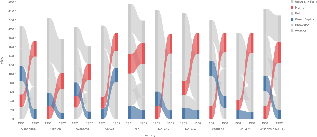
connect related bars

layer([
  chart(barley)
    .flow(
      spread(by="variety", dir="x", spacing=24),
      spread(by="year", dir="x", spacing=16),
      stack(by=field("site").sort("yield"), dir="y", size="yield")
    )
    .mark(rect(w=8, fill="site").name("bars")),
  chart(selectAll("bars"))
    .flow(group(by="variety"), group(by="site"))
    .mark(ribbon(opacity=0.5))
])

style is downstream of structure

layer([
  chart(barley, color=palette({
    "Waseca": "#d7dadd", "Morris": "#49a66a",
    "Grand Rapids": "#d7dadd",
    "Crookston": "#d7dadd", "Duluth": "#d7dadd",
  }))
    .flow(
      spread(by="variety", dir="x", spacing=38),
      spread(by="year", dir="x", spacing=8),
      stack(by=field("site").sort("yield"), dir="y", size="yield")
    )
    .mark(rect(w=16, fill="site").name("bars")),
  chart(selectAll("bars"))
    .flow(group(by="variety"), group(by="site"))
    .mark(ribbon(opacity=0.78))
])

mapping length to angle changes the afforded queries

pie

bar

Fine-grained comparison is MUCH harder

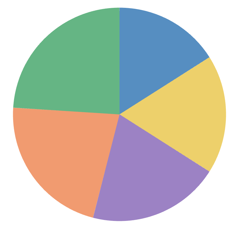
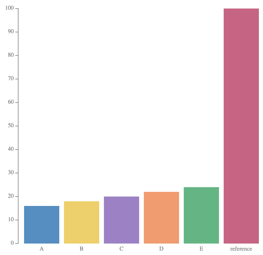
mapping length to angle changes the afforded queries

pie

bar

But coarse part-to-whole comparisons are much easier!

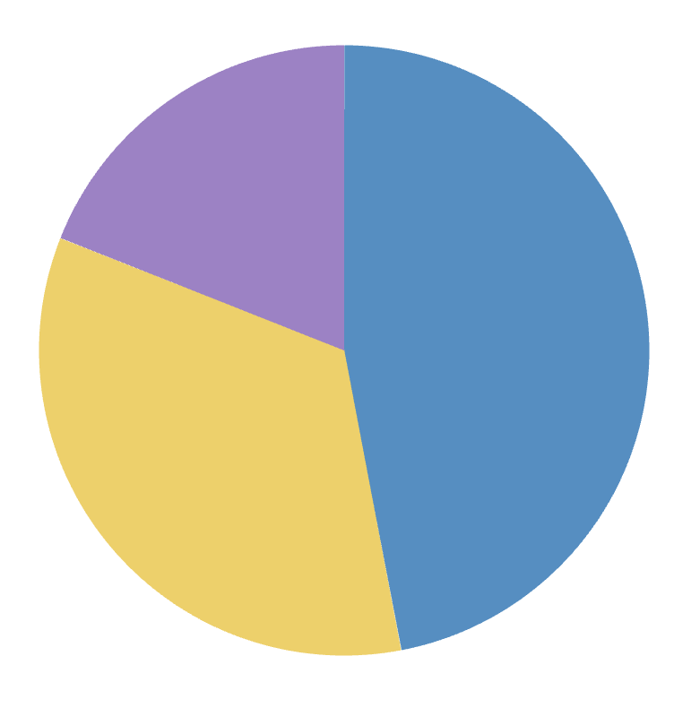
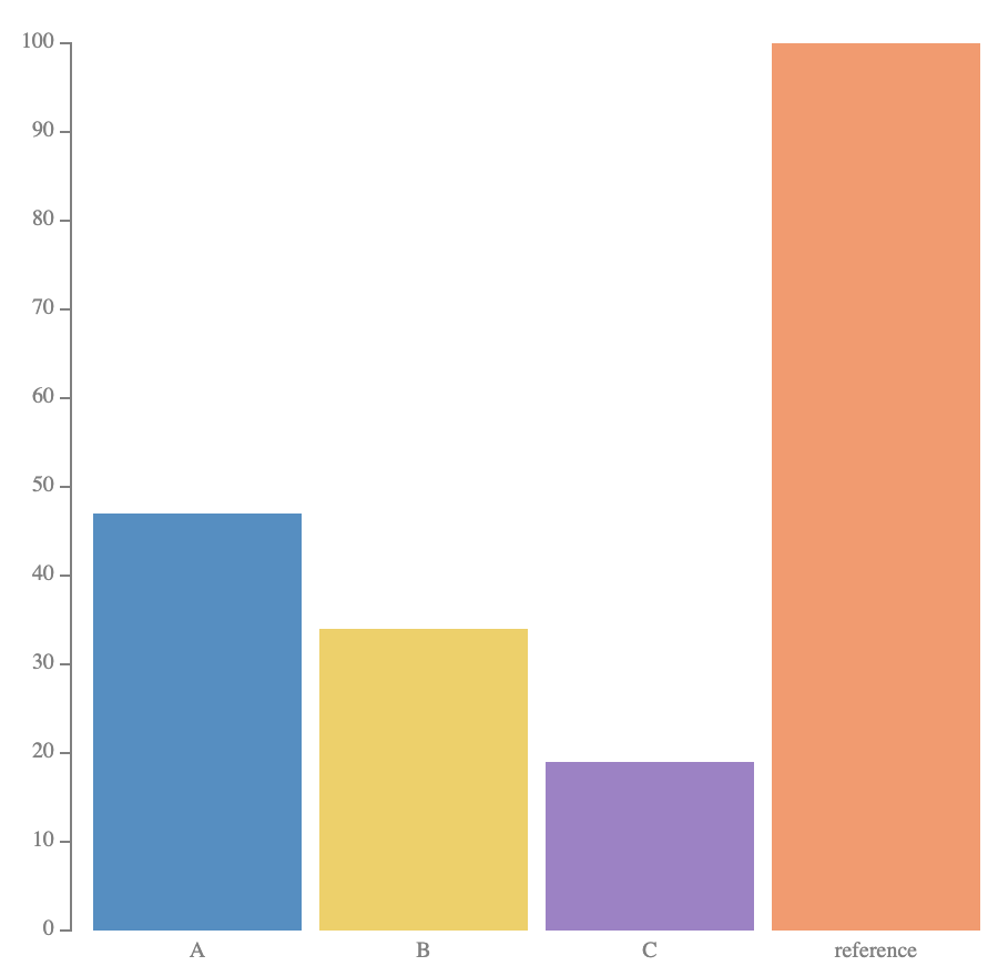
scatter -> pie = scatterpie

chart(scatter_data).flow(
    scatter(by="lake", x="x", y="y")
).mark(
    chart(coord=clock())
    .flow(stack(by="species", dir="x", size="count"))
    .mark(rect(fill="species"))
)

Outer structure: scatter() affords "where?" queries.

Inner structure: pie affords "what fraction?" queries.

Queries:

which species dominates each lake? (largest slice)
how does species composition vary across geography?
which lakes have similar mixes? (visual comparison)

same glyph, new dataset: barley, two years

# x, y: each site's Minnesota lon/lat
def site_pie(data):
    total_yield = total_yield_for(1931, data[0]["site"])
    return (
        chart(data[0]["collection"], coord=clock())
        .flow(stack(by="variety", dir="x", h=pie_radius(total_yield), size="yield"))
        .mark(rect(fill="variety"))
    )

chart(barley_scatter_by_year(1931)).flow(
    scatter(by="site", x="x", y="y")
).mark(site_pie)

Same construction as the lake scatter-pie: each trial site sits at its real Minnesota location, and each glyph is a pie of that site's variety mix.

New move: pie radius (h) scales with each site's total yield that year, on a shared scale across both charts.

Watch Morris:

every other site's pie shrinks from 1931 → 1932, Morris's grows
radius affords the magnitude query the seafood version couldn't; angle still affords the mix query

1931

1932

This is the famous Minnesota barley anomaly (Fisher/Immer data, popularized by Cleveland & via the trellis-display literature): nearly every site's yield fell from 1931 to 1932, except Morris, which rose. The pies sit at each site's actual geography, Crookston in the far northwest, Duluth on Lake Superior in the northeast, Waseca in the south, Morris mid-west, so the chart doubles as a map of Minnesota. Encoding total yield as pie radius (instead of a fixed radius, as in the lake version) makes the flip visible at a glance without giving up the proportion read inside each pie. Same outer/inner grammar as the seafood scatter-pie, only the radius channel is new.

first, just the points

find ⟨each variety's trend⟩ at each site, one variety, or all?

chart(barley)
  .flow(
    spread(by="site", dir="x"),
    spread(by="year", dir="x"),
    scatter(by="variety", y="yield")
  )
  .mark(circle(r=3, fill="variety"))

connect the points with lines

find ⟨each variety's trend⟩ at each site, one variety, or all?

chart(barley)
  .flow(
    spread(by="site", dir="x"),
    spread(by="year", dir="x"),
    scatter(by="variety", y="yield"),
  )
  .mark(line(by="variety", along="year", fill="variety"))

In the grouped bars, each variety's years were finally adjacent, but the change still had to be estimated between two tiny bar heights. Here the line makes that relation a single trajectory. Spread still creates the six site panels and the two year positions. Scatter creates one entity per variety, and line connects that variety's two values. One quantifier, site, is a scan across panels. The other, variety, is a scan down each panel's ten lines. The sign predicate reads from each line's slope. This is Trellis-style: Becker and Cleveland's own display for this dataset. It preserves both absolute yields and each year-to-year trajectory, but the reader still has to aggregate ten slope signs per panel to recover the sentence. The delta bars ahead trade away those endpoints and trajectories so every signed change can share one positional baseline.

for change, position beats angle

Slope gives direction immediately. But comparing how much each variety changed means comparing line angles.

Delta bars put every signed change against the same zero baseline. We give up the two absolute yields and the explicit trajectory.

simplify your message

find ⟨each variety's trend⟩ at each site, one variety, or all?

chart(barley)
  .flow(
    spread(by="site", dir="x"),
    spread(by="year", dir="x"),
    scatter(by="variety", y="yield"),
  )
  .mark(line(stroke="variety"))

anchor the comparison

compare ⟨Δ yield from 1931⟩, site by site

chart(barley)  .flow(    derive(anchor_to_1931),    spread(by="site", dir="x"),    spread(by="year", dir="x"),    scatter(by="variety", y="delta_from_1931"),  )  .mark(line(stroke="variety"))

trade angle for position

find ⟨the sign of Δ yield⟩, by site

chart(barley)  .flow(    spread(by="site", dir="x"),    spread(by="variety", dir="x"),    derive(lambda rows: [{      **rows[0], "delta": rows[1]["yield"] - rows[0]["yield"]    }]),  )  .mark(rect(h="delta"))

the line has nothing left to connect

chart(barley)  .flow(    derive(delta),    spread(by="site", dir="x"),    scatter(by="variety", y="delta"),  )  .mark(circle(r=4))

use color for emphasis

find ⟨the sign of Δ yield⟩, by site

chart(barley, color=palette({"Morris": "#e08214"}))
  .flow(
    spread(by="site", dir="x"),
    spread(by="variety", dir="x"),
    derive(lambda rows: [{
      **rows[0], "delta": rows[1]["yield"] - rows[0]["yield"]
    }]),
  )
  .mark(rect(h="delta", fill="site"))

Identical to the previous delta-bars slide, but the bars are now filled by site through a Morris-orange palette; everything else goes gray. This is deliberately late in the arc: the sign question was already answered structurally (bar direction from a zero baseline), so color isn't recruited to encode sign, it only has to say "look here." That's the whole point of moving color to this slide instead of the slope chart: on the slope panels color would have had to do two jobs (which lines are which site, and which site to look at) where here it only has one. Own it honestly on stage: GoFish has no `emphasize()` primitive yet. What's on screen is a hand-written conditional in the render function (`highlight ? palette(...) : the default color scale`), not a first-class operator, filed as gofish#641, and worth fixing precisely because "highlight one category, gray out the rest" is common enough to deserve its own name instead of a per-chart if/else.

annotations can emphasize your message

find ⟨the sign of Δ yield⟩, by site

proposed in #805

chart(barley, color=palette({"Morris": "#e08214"}))  .flow(    spread(by="site", dir="x")      .label(        field("site").map({          "Morris": "Only Morris rose across every variety"        }),        position="outset-top", color="#e08214"      ),    spread(by="variety", dir="x"),    derive(lambda rows: [{      **rows[0], "delta": rows[1]["yield"] - rows[0]["yield"]    }]),  )  .mark(rect(h="delta", fill="site"))

The last step of explanatory polish: annotate. If the sentence is the point, write the sentence on the chart, don't leave the reader to reconstruct it from a color cue alone. Same delta bars, same Morris-orange highlight, color already made Morris's bars pop; the callout states the conclusion directly instead of leaving the reader to scan six site groups of signed bars. The visible code is the proposed field-map spelling from draft PR #805: it is a serializable partial mapping, and an unmapped value produces no label. Until that PR lands, this live chart uses the already-merged equivalent: a derived takeaway field that is empty for five sites and contains the sentence for Morris, labeled on the outer site spread. Exploratory charts help you find the story; explanatory charts tell it.

Swap the inner chart for a different part-to-whole viz

FLOWER_RADIUS = 40
stem_data = [{**d, "x": catch_locations[d["lake"]]["x"]} for d in seafood]

layer([
  chart(stem_data)
    .flow(scatter(by="lake", x="x"))
    .mark(
      rect(w=4, h="count", fill=color.green[5])
        .name("stems")
    ),
  chart(selectAll("stems"))
    .flow(group(by="lake"))
    .mark(lambda d: spread(
        [
          d[0],
          layer([
            stackX(
              [
                petal(w=v(r["count"]), fill=v(r["species"]).lighten(0.5))
                for r in d[0]["datum"]
              ],
              h=FLOWER_RADIUS, spacing=0,
              alignment="start", sharedScale=True,
            ),
          ], coord=polar()),
        ],
        dir="y", alignment="middle",
        spacing=-FLOWER_RADIUS,
    )),
])

balloons???

def balloon(x, y, scale, colors):
  return Frame(
    [
      ellipse(cx=15, cy=15, w=24, h=30, fill=colors["body"]),
      ellipse(cx=12, cy=11, w=7, h=11, fill=colors["highlight"]),
      rect(cx=15, cy=32, w=8, h=4,
        fill=colors["knot"], rx=3, ry=2),
      rect(cx=15, cy=32, w=5, h=2.4,
        fill=colors["knot"], rx=2, ry=1),
    ],
    x=x - 15 * scale,
    y=y + 27 * scale,
    box=True,
    transform={"scale": {"x": scale, "y": -scale}},
  )


def balloon_for_sample(sample):
  top3 = sorted(
    sample["collection"],
    key=lambda r: r["count"],
    reverse=True,
  )[:3]

  return Frame([
    rect(x=0, y=0, w=1, h=sample["y"], emY=True),
    balloon(0, sample["y"], 1, {
      "body": species_color_map[top3[0]["species"]],
      "highlight": species_color_map[top3[1]["species"]],
      "knot": species_color_map[top3[2]["species"]],
    }),
  ], x=sample["x"])


Frame(
  [balloon_for_sample(sample) for sample in scatter_by_lake],
  coord=wavy(), x=0, y=0,
)

TODO Python: expose a balloon glyph helper with body, highlight, and knot channels.

When we think with structure instead of chart types, we can move between the familiar charts from first principles.

An example gallery helps when you already know what you want. Structure helps when you don't.

What just happened?

We took one dataset and made a series of deliberate structural moves.

Each move changed what was easy or hard to see.

We didn't have to pick from a menu of charts... though those are useful shorthands for common structures!

Instead, chart type labels like bar or pie were just structural motifs we encountered along the way.

choose by the structure you need

What you want to see	Operator	Visual structure
compare the same measure across discrete groups	`spread(by=key)`
see how parts add up to a whole	`stack(by=key, size=value)`
see how two measures vary together	`scatter(by=key, x=x, y=y)`
follow the same item across positions	`line(by=key)` or `ribbon(by=key)`
look up a value by two discrete keys	`table(by=(row, col))`

Beyond layout: data transforms change the values, color changes grouping and emphasis, and coordinate transforms change the geometry.

each operator makes one query cheap

Operator	shape	index what `by=` builds	ask the queries it makes cheap
`spread(by=key)`	1 axis · discrete	`key → its own slot`, side by side	look up ⟨an entity⟩ at its key compare ⟨summaries⟩ across key
`stack(by=key, size=value)`	1 axis · discrete · slots sized by value	`key → a segment sized by value`, tiled end to end in order	look up ⟨key's segment⟩ in order compare ⟨sizes⟩ across key read ⟨the total = Σ size⟩ at the far edge
`scatter(by=key, x=x, y=y)`	1–2 axes · continuous	`key → a point at (x, y)`	look up ⟨an entity⟩ at (x, y) collect ⟨the shape of the crowd⟩
`table(by=(row, col))`	2 axes · discrete	`(row, col) → a cell`, a grid both ways	look up ⟨a value⟩ at (row, col) compare ⟨…⟩ along a row or a column
relational, draws over an index, builds none
`line() / ribbon()`	no index, draws over one	none	follow ⟨an entity⟩ across scopes read ⟨crossings⟩ as overtakes

queries after Brehmer & Munzner (2013)

spread, discrete; alignment & uniform density.
stack, partitioned continuous; part-to-whole.
scatter, continuous × continuous; proximity.
area / line / ribbon, continuous or contiguous; connection.
table, discrete × discrete; uniform density.

Every operator does two jobs: an addressing move (what's where, what's locatable) and a pricing move (which readings become one perceptual act). Connection is the only pure pricing move, and the scatterpie works by keeping scatter's addressing while swapping the value payload.

The scatterpie composes two of these: scatter contributes how the distribution varies across space, the pie glyph contributes share-within-entity.

Connection is the strongest grouping cue there is, stronger than proximity, stronger than color or shape similarity (Franconeri, Bemis, Burlingham & Kramer 2021, PSPI, Fig. 8). Explicit connecting lines improve relation judgments by 25–95% (Nothelfer & Franconeri 2020). Note this is a strength ranking, not Palmer & Rock's 1994 claim about processing priority (which is about order of computation, not which cue wins).

That ranking is a default, not a total order: connection > common region/connectedness > proximity > similarity (color > shape). Cue strength is parametric and cues combine additively in log-odds (Kubovy & van den Berg 2008; Brooks 2015), so a strong enough similarity cue can override a weak proximity cue (Quinlan & Wilton 1998). In grouped bar charts specifically, spatial proximity beats color grouping for comparisons about 63/37 of the time (Bearfield, Stokes, Lovett & Franconeri 2024, TVCG). Full notes: notes/gestalt-grouping-strength.md.

The bottom line about color is the nonlocal grouping cue: similarity groups marks without adjacency and without building a spatial index, no by= to point to. By default it sits below proximity in the strength ranking above, but that ordering is parametric, not fixed: a large enough color difference, or tight enough spacing, can flip it (same Quinlan & Wilton 1998 / Bearfield et al. 2024 point as above, applied to this table's own operators).

the ask column's verbs are Brehmer & Munzner's: look up and follow are their search actions, compare/read/collect their query actions. Their identify/compare/summarize ladder maps onto this table three ways: identify is a mark-level read, compare is the operator's ask line, summarize is what the hole collapses down to once a scope docks upward, worth saying out loud, since the chip no longer prints a price for it.

spread is align + distribute: distribute builds the index (the index cell, one slot per key), align prices the comparison itself (the ask line). Which align anchor you pick decides which comparison is precise: baseline anchoring gives common-scale length comparisons, middle anchoring gives symmetric deviation comparisons.

stack trades per-key comparison accuracy, interior segments lose the shared baseline the moment they're not first, for a free read of the total at the far edge. That far edge, Σ size, is itself a size an enclosing operator can consume. Normalize it (size: field(...).normalize()) and the far edge reads as ⟨each key's share⟩ instead of an absolute total.

scatter's key is one field, with x/y carried as attributes (by= is optional, omit it for a per-item scatter). A 1D scatter, with only x or only y bound, is a strip plot, hence "1–2 axes" under the preview. table's key is two fields crossed (by={row, col}); that row/col split is what makes it discrete both ways, versus scatter's continuous one-or-two.

⟨the shape of the crowd⟩ = trends, clusters, outliers, the gestalt reads a scatter affords for free. Scagnostics is the formalization of exactly that list.

What each operator's "places" used to say, before the shape column replaced the prose: spread, one slot per value of a field. stack, scopes tiled end to end; boundaries at the running totals. scatter, each entity at its location in space. area / line / ribbon, nothing new; draws over existing placements. table, two independently addressable axes.

beyond standard charts

move 1 of 4 · bars → pies → scatter

shares as stacked bars

compare ⟨species shares⟩ across lakes

→

the same shares as pies

compare ⟨species shares⟩ across lakes

→

which species dominates each lake?

compare ⟨species shares⟩ across lakes at ⟨their places in space⟩

beyond standard charts

size → units

the same counts as continuous bars

compare ⟨species shares, as segments⟩ across lakes

→

how many fish, exactly?

compare ⟨species shares, as countable squares⟩ across lakes

continuous bars

chart(seafood)
  .flow(
    spread(by="lake", dir="x"),
    stack(by="species", dir="y", size="count")
  )
  .mark(rect(w=36, fill="species"))

countable units

chart(seafood)
  .flow(
    spread(by="lake", dir="x"),
  )
  .mark(waffle(count="count", fill="species"))

waffle mark

def waffle(count, fill, columns=5):
  return flow(
    repeat(count), chunk(columns),
    spread(dir="y", reverse=True), spread(dir="x"),
  ).mark(rect(w=8, h=8, fill=fill))

beyond standard charts

one more level

did third class fare better than crew?

compare ⟨survival shares⟩ across classes

→

condition on sex: the answer flips

compare ⟨survival shares⟩ across class × sex

one level

chart(titanic)
  .flow(
    stack(by="class", dir="y", size=field("count").normalize()),
    stack(by="survived", dir="x", size=field("count").normalize())
  )
  .mark(rect(fill="survived"))

one more level

chart(titanic)
  .flow(
    stack(by="class", dir="y", size=field("count").normalize()),
    stack(by="sex", dir="x", size=field("count").normalize()),
    stack(by="survived", dir="y", size=field("count").normalize())
  )
  .mark(rect(fill="survived"))

beyond standard charts

sort + connect

each year's stack, sorted

compare ⟨source shares⟩ within a year

connect

→

the same stacks, connected

follow ⟨each source⟩ across years

sort + connect

→

which source overtook which?

sources sorted by amount, each year follow ⟨each source⟩ across years read ⟨crossings⟩ as overtakes

sort each year's stack

sorted = chart(energyMix)
  .flow(spread(by="year", dir="x"),
    stack(by=field("source").sort("amount"), dir="y"))
  .mark(rect(h="amount", fill="source"))

connect the stacks

area = chart(energyMix)
  .flow(spread(by="year"), stack(by="source"))
  .mark(ribbon(by="source", h="amount", fill="source", opacity=0.8))

sort + connect

chart(energyMix)
  .flow(
    spread(by="year", dir="x"),
    stack(by=field("source").sort("amount"), dir="y")
  )
  .mark(rect(h="amount", fill="source"))
  .layer(ribbon(by="source", opacity=0.5))

UK electricity generation · Our World in Data / Ember

Third move, in three stages. First, sort each year's stack by amount: rank reads as position, but sorting re-purposes position from an identity channel to a rank channel, so following one source across years is a color hunt. Then connect instead: the bands carry "same source" identity across years, but in fixed stacking order they never cross, so there's nothing to read at a crossing. Compose them and the combination pays off: with rank as position AND identity as continuity, a crossing IS a rank inversion, an overtake event, read directly. Real data: UK share of electricity generation (Our World in Data / Ember). Wind passes Coal between 2014 and 2018, Coal collapses 29.6% to 5.0%, so Nuclear passes it too, then Wind passes Nuclear between 2018 and 2022, and Solar passes Coal by 2022: renewables overtaking legacy sources one crossing at a time. Contrast with the barley walkthrough this replaced: there the story was sign-of-change (did each variety rise or fall?), and the ribbon answered an adjacent rank question, the slope panels carry that beat now. Rank change is the query ribbons are actually FOR, so the ribbon lives here.

beyond standard charts

pictorial charts

ordinary normalized bars

→

paint the bars as bottles

→

layer on labels

normalized bars

chart(bottleData, axes=False)
  .flow(spread(by="category", dir="x", spacing=20))
  .mark(layer([
    rect(h=datum(100), fill="gray"),
    rect(h="amount", fill="green"),
  ]))

paint the bottle

chart(bottleData, axes=False)
  .flow(spread(by="category", dir="x", spacing=20))
  .mark(paint([
    image(href=bottlePng, h=datum(100)),
    rect(h="amount", w=175, fill="green"),
  ], blendMode="color"))

layer on labels

chart(bottleData, axes=False)
  .flow(spread(by="category", dir="x", spacing=20))
  .mark(
    layer([
      paint([
        image(href=bottlePng, h=datum(100)),
        rect(h="amount", w=175, fill="green"),
      ], blendMode="color").name("bottle"),
      rect(h=1, y="amount", fill="gray").name("line"),
      text(text="{amount}%", fill="gray").name("label"),
    ]).constrain(lambda bottle, line, label: [
      Constraint.align([bottle, line], x="start"),
      Constraint.distribute([line, label], dir="y", spacing=0),
      Constraint.align([label, line], x="end"),
    ])
  )

Pictorial composition grammar adapted from PiCCL · Shi et al., IEEE VIS 2025

three stacks make a mosaic

chart(titanic)
  .flow(
    stack(by="class",    dir="y", size=field("count").normalize()),
    stack(by="sex",      dir="x", size=field("count").normalize()),
    stack(by="survived", dir="y", size=field("count").normalize())
  )
  .mark(
    rect(fill="survived")
  )

Crew

Third

Second

First

women

men

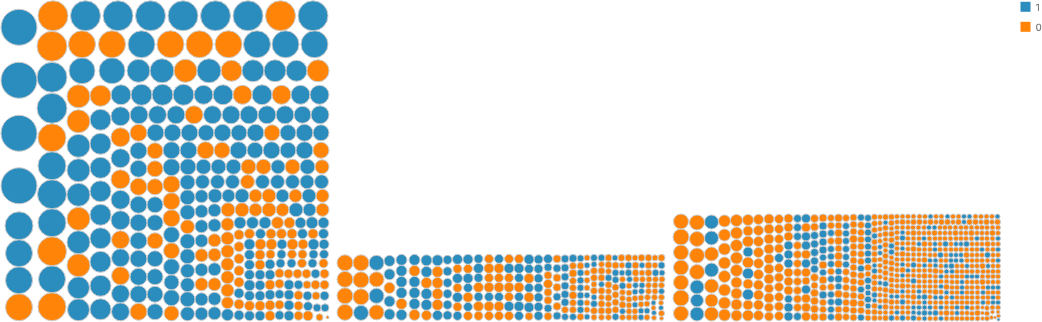
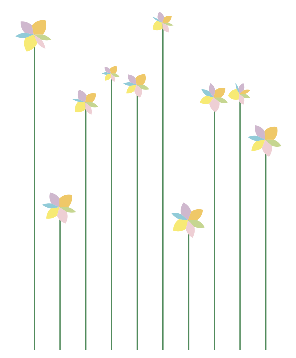
the same moves, stranger structures

Polar ribbon chart with five colored ribbons wrapping and crossing around a circular coordinate system

Insertion sort trace with five array stages, sorted-prefix outlines, and arrows showing each move

Multilevel silhouette tree mixing radial node-link fans and filled wedge silhouettes

Layered bars and area chart showing barley yield changes between 1931 and 1932 across varieties

Titanic fare circle treemap with passengers packed by class, sized by fare, and colored by survival

Flower chart with multicolored petals showing species counts for each lake

Escalation beat. The moves the audience just learned, spread, stack, nest, restyle, don't stop where the chart menu does. Walk the six examples: polar ribbon, insertion sort, multilevel silhouette tree, layered bars and area, Titanic fare circle treemap, and flower chart. Each pushes a familiar operation further: wrap and connect; align and constrain; switch templates inside a hierarchy; layer bars with ribbons; pack circles by fare; replace bars with multivariate glyphs. They are not six new primitive chart types. They are the same small structural vocabulary composed in six different ways. [advance] Keep composing the same moves and you run out of chart names.

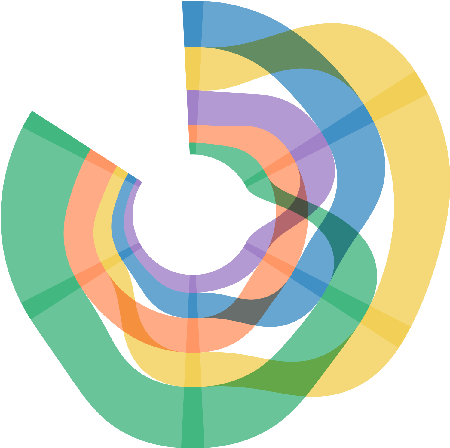
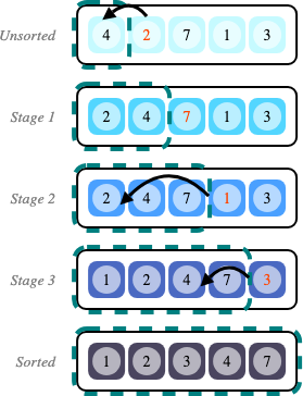
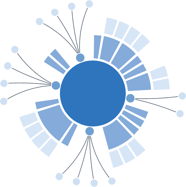
Why "more"

a grammar of more graphics

The Grammar of Graphics fits inside GoFish, and so do grammars beyond it.

GoFish's own test gallery reimplements, example by example:

vega-lite: the grammar underneath Altair
Atom: unit & dot-plot charts
PiCCL: pictorial charts (the bottle)
GoTree: a tree-layout grammar, 46 gallery examples
seaborn-style jointplots, and Bluefish diagrams

takeaways

1. Graphics are visual data structures that we query with our eyes.

2. GoFish makes visual structure composable, letting us build familiar charts and continue beyond what conventional visualization grammars make easy.

3. Start with what the reader needs to see, then build the structure that makes it easy.

Try it

$pip install --pre gofish-graphics

Python alpha release is here!

🌐 Docs: gofish.graphics

🐙 GitHub: gofish-graphics/gofish-graphics

🎞️ Slides: gofish-graphics/scipy-2026-talk

find me

joshmpollock.com

🐦 X: @joshmpollock

🐙 GitHub: @joshpoll

💼 LinkedIn: joshmpollock

✉️ Email: jopo@mit.edu

what's next?

I’m defending my PhD in a week and a half(!) I don’t know exactly what comes next, but I want to work with scientists, mathematicians, and software engineers on challenging visualization design problems. I also want to maintain GoFish as a system that bridges visualization research and practice.

GoFish: Graphical Structure in Plain Sight

you can one-shot a dashboard now

…or even a scrollytelling narrative

ok, but is it actually good?

we need to see structure, not chart types

start with the lakes

how do we decide what chart to use?

how do we decide what chart to use?

how do we decide what chart to use?

how do we decide what chart to use?

menus become rules

and often that's fine

but what about the long tail

I'm a stylistic anarchist

grammar vs elements of style

Grammar

Style

graphics don't always fall into neat taxonomies

here's a grouped bar chart

what did you notice about the data?

here's another one

what did you notice now?

what about now?

how about now?

these are all grouped bar charts, but we read them differently!

by the way: this is real data

the grammar of graphics: marks, channels, and coordinates

marks (shapes)

channels (shape attributes)

coordinates (space transformations)

but we need a notion of visual structure to explain what we just saw

graphics are visual data structures 🪾

that we query with our eyes 👀

so we need two languages

GoFish

visual structure can help us describe both simple charts and very complex ones

familiar chart space

the long tail

beyond chart space

high fashion for graphics tools

GoFish is based on Gestalt grouping principles

GoFish has three four API tiers

back to those bar charts

start with the data shape

start with the data

place one slot per site

make yield visible

some transforms are implied

add a second grouping

data transformation pipeline

each line of the spec is a cut

each line of the spec is a cut

each line of the spec is a cut

group by site, then year

or group by year, then site

nesting order changes the question

site → variety

variety → site

is it one variety, or all of them?

just spread again?

stack()

did the mix change?

now sort each normalized stack

same question, as pies

flattening the hierarchy

sort() on the stack

sort each stack

connect related bars

style is downstream of structure

mapping length to angle changes the afforded queries

mapping length to angle changes the afforded queries

scatter -> pie = scatterpie

same glyph, new dataset: barley, two years

first, just the points

connect the points with lines

for change, position beats angle

simplify your message

anchor the comparison

trade angle for position

the line has nothing left to connect

`stack()`

`sort()` on the stack